论文阅读笔记:Denoising Diffusion Implicit Models (4)
0、快速访问
论文阅读笔记:Denoising Diffusion Implicit Models (1)
论文阅读笔记:Denoising Diffusion Implicit Models (2)
论文阅读笔记:Denoising Diffusion Implicit Models (3)
论文阅读笔记:Denoising Diffusion Implicit Models (4)
4、接上文[论文阅读笔记:论文阅读笔记:Denoising Diffusion Implicit Models (3)
- 已经知道跳 1 1 1步时, q σ ( x t − 1 ∣ x t , x 0 ) q_{\sigma}(x_{t-1}|x_t,x_0) qσ(xt−1∣xt,x0)的分布满足公式(·)
x t − 1 = α t − 1 ⋅ x t − 1 − α t ⋅ z t α t + 1 − α t − 1 ⋅ z t \begin{equation} \begin{split} x_{t-1}&=\sqrt{\alpha_{t-1}} \cdot \frac{x_t-{\sqrt{1-\alpha_t}\cdot z_t}}{\sqrt{\alpha_t}} + \sqrt{1-\alpha_{t-1}}\cdot z_t\\ \end{split} \end{equation} xt−1=αt−1⋅αtxt−1−αt⋅zt+1−αt−1⋅zt - 假设跳 n n n步时, q σ ( x t − n ∣ x t , x 0 ) q_{\sigma}(x_{t-n}|x_t,x_0) qσ(xt−n∣xt,x0)的分布满足公式(2)
x t − n = α t − n ⋅ x t − 1 − α t ⋅ z t α t + 1 − α t − n ⋅ z t \begin{equation} \begin{split} x_{t-n}&=\sqrt{\alpha_{t-n}} \cdot \frac{x_t-{\sqrt{1-\alpha_t}\cdot z_t}}{\sqrt{\alpha_t}} + \sqrt{1-\alpha_{t-n}}\cdot z_t\\ \end{split} \end{equation} xt−n=αt−n⋅αtxt−1−αt⋅zt+1−αt−n⋅zt - 证明:当跳 n + 1 n+1 n+1步时,分布 q σ ( x t − n − 1 ∣ x t , x 0 ) q_{\sigma}(x_{t-n-1}|x_t,x_0) qσ(xt−n−1∣xt,x0)满足 x t − n − 1 = α t − n − 1 ⋅ x t − 1 − α t ⋅ z t α t + 1 − α t − n − 1 ⋅ z t x_{t-n-1}=\sqrt{\alpha_{t-n-1}} \cdot \frac{x_t-{\sqrt{1-\alpha_t}\cdot z_t}}{\sqrt{\alpha_t}} + \sqrt{1-\alpha_{t-n-1}}\cdot z_t xt−n−1=αt−n−1⋅αtxt−1−αt⋅zt+1−αt−n−1⋅zt。
由于 q σ ( x t − n − 1 ∣ x t , x 0 ) q_{\sigma}(x_{t-n-1}|x_t,x_0) qσ(xt−n−1∣xt,x0)是 q σ ( x t − n − 1 , x t − n ∣ x t , x 0 ) q_{\sigma}(x_{t-n-1},x_{t-n}|x_t,x_0) qσ(xt−n−1,xt−n∣xt,x0)的边缘分布,因此有
q σ ( x t − n − 1 ∣ x t , x 0 ) = ∫ q σ ( x t − n − 1 , x t − n ∣ x t , x 0 ) ⋅ d x t − n = ∫ q σ ( x t − n − 1 , ∣ x t − n , x 0 ) ⋅ q σ ( x t − n ∣ x t , x 0 ) ⋅ d x t − n \begin{equation} \begin{split} q_{\sigma}(x_{t-n-1}|x_t,x_0)&=\int q_{\sigma}(x_{t-n-1},x_{t-n}|x_t,x_0) \cdot dx_{t-n} \\ &=\int q_{\sigma}(x_{t-n-1},|x_{t-n},x_0) \cdot q_{\sigma}(x_{t-n}|x_t,x_0) \cdot dx_{t-n} \end{split} \end{equation} qσ(xt−n−1∣xt,x0)=∫qσ(xt−n−1,xt−n∣xt,x0)⋅dxt−n=∫qσ(xt−n−1,∣xt−n,x0)⋅qσ(xt−n∣xt,x0)⋅dxt−n
q σ ( x t − n − 1 , ∣ x t − n , x 0 ) = N ( x t − n − 1 ∣ 1 − α t − n − 1 1 − α t − n ⋅ x t − n + [ α t − n − 1 − α t − n ⋅ ( 1 − α t − n − 1 ) 1 − α t − n ] ⋅ x 0 , 0 ) q_{\sigma}(x_{t-n-1},|x_{t-n},x_0)=N\bigg(x_{t-n-1}|\sqrt{\frac{1-\alpha_{t-n-1}}{1-\alpha_{t-n}}}\cdot x_{t-n}+ \bigg[\sqrt{\alpha_{t-n-1}}- \frac{\sqrt{ \alpha_{t-n}\cdot (1-\alpha_{t-n-1}} )}{\sqrt{1-\alpha_{t-n}}} \bigg] \cdot x_0, 0\bigg) qσ(xt−n−1,∣xt−n,x0)=N(xt−n−1∣1−αt−n1−αt−n−1⋅xt−n+[αt−n−1−1−αt−nαt−n⋅(1−αt−n−1)]⋅x0,0)
因此,分布 q σ ( x t − n − 1 ∣ x t , x 0 ) q_{\sigma}(x_{t-n-1}|x_t,x_0) qσ(xt−n−1∣xt,x0)的均值 μ t − n − 1 \mu_{t-n-1} μt−n−1如公式(4)所示。
μ t − n − 1 = E ( q σ ( x t − n − 1 ∣ x t , x 0 ) ) = ∫ x t − n − 1 ⋅ q σ ( x t − n − 1 ∣ x t , x 0 ) ⋅ d x t − n − 1 = ∫ x t − n − 1 ⋅ ( ∫ q σ ( x t − n − 1 , ∣ x t − n , x 0 ) ⋅ q σ ( x t − n ∣ x t , x 0 ) ⋅ d x t − n ) ⋅ d x t − n − 1 = ∫ ∫ x t − n − 1 ⋅ q σ ( x t − n − 1 , ∣ x t − n , x 0 ) ⋅ q σ ( x t − n ∣ x t , x 0 ) ⋅ d x t − n ⋅ d x t − n − 1 = ∫ ( ∫ x t − n − 1 ⋅ q σ ( x t − n − 1 , ∣ x t − n , x 0 ) ⋅ d x t − n − 1 ) ⋅ q σ ( x t − n ∣ x t , x 0 ) ⋅ d x t − n = ∫ E ( q σ ( x t − n − 1 , ∣ x t − n , x 0 ) ) ⋅ q σ ( x t − n ∣ x t , x 0 ) ⋅ d x t − n = ∫ ( 1 − α t − n − 1 1 − α t − n ⋅ x t − n + [ α t − n − 1 − α t − n ⋅ ( 1 − α t − n − 1 ) 1 − α t − n ] ⋅ x 0 ) ⋅ q σ ( x t − n ∣ x t , x 0 ) ⋅ d x t − n = ∫ 1 − α t − n − 1 1 − α t − n ⋅ x t − n ⋅ q σ ( x t − n ∣ x t , x 0 ) ⋅ d x t − n + ∫ ( [ α t − n − 1 − α t − 1 ⋅ ( 1 − α t − n − 1 ) 1 − α t − n ] ⋅ x 0 ) ⋅ q σ ( x t − n ∣ x t , x 0 ) ⋅ d x t − n = 1 − α t − n − 1 1 − α t − n ⋅ ∫ q σ ( x t − n ∣ x t , x 0 ) ⋅ d x t − n + [ α t − n − 1 − α t − n ⋅ ( 1 − α t − n − 1 ) 1 − α t − n ] ⋅ x 0 = 1 − α t − n − 1 1 − α t − n ⋅ E ( q σ ( x t − n ∣ x t , x 0 ) ) + [ α t − n − 1 − α t − n ⋅ ( 1 − α t − n − 1 ) 1 − α t − n ] ⋅ x 0 ⏟ x 0 = x t − 1 − α t ⋅ z t α t = 1 − α t − n − 1 1 − α t − n ⋅ ( α t − n ⋅ x t − 1 − α t ⋅ z t α t + 1 − α t − n ⋅ z t ) + [ α t − n − 1 − α t − n ⋅ ( 1 − α t − n − 1 ) 1 − α t − n ] ⋅ x t − 1 − α t ⋅ z t α t = 1 − α t − n − 1 1 − α t − n ⋅ α t − n ⋅ x t − 1 − α t ⋅ z t α t + 1 − α t − n − 1 1 − α t − n ⋅ 1 − α t − n ⋅ z t + α t − n − 1 ⋅ x t − 1 − α t ⋅ z t α t − α t − n ⋅ ( 1 − α t − n − 1 ) 1 − α t − n ⋅ x t − 1 − α t ⋅ z t α t = α t − n − 1 ⋅ x t − 1 − α t ⋅ z t α t + 1 − α t − n − 1 ⋅ z t \begin{equation} \begin{split} \mu_{t-n-1}&=E\big(q_{\sigma}(x_{t-n-1}|x_t,x_0) \big)\\ &=\int x_{t-n-1}\cdot q_{\sigma}(x_{t-n-1}|x_t,x_0) \cdot dx_{t-n-1} \\ &=\int x_{t-n-1}\cdot \bigg(\int q_{\sigma}(x_{t-n-1},|x_{t-n},x_0) \cdot q_{\sigma}(x_{t-n}|x_t,x_0) \cdot dx_{t-n} \bigg) \cdot dx_{t-n-1} \\ &=\int \int x_{t-n-1}\cdot q_{\sigma}(x_{t-n-1},|x_{t-n},x_0) \cdot q_{\sigma}(x_{t-n}|x_t,x_0) \cdot dx_{t-n} \cdot dx_{t-n-1} \\ &=\int \bigg( \int x_{t-n-1}\cdot q_{\sigma}(x_{t-n-1},|x_{t-n},x_0) \cdot dx_{t-n-1}\bigg) \cdot q_{\sigma}(x_{t-n}|x_t,x_0) \cdot dx_{t-n} \\ &=\int E\big(q_{\sigma}(x_{t-n-1},|x_{t-n},x_0) \big) \cdot q_{\sigma}(x_{t-n}|x_t,x_0) \cdot dx_{t-n} \\ &=\int \bigg(\sqrt{\frac{1-\alpha_{t-n-1}}{1-\alpha_{t-n}}}\cdot x_{t-n}+ \bigg[\sqrt{\alpha_{t-n-1}}- \frac{\sqrt{ \alpha_{t-n}\cdot (1-\alpha_{t-n-1}} )}{\sqrt{1-\alpha_{t-n}}} \bigg] \cdot x_0 \bigg) \cdot q_{\sigma}(x_{t-n}|x_t,x_0) \cdot dx_{t-n} \\ &=\int \sqrt{\frac{1-\alpha_{t-n-1}}{1-\alpha_{t-n}}}\cdot x_{t-n} \cdot q_{\sigma}(x_{t-n}|x_t,x_0) \cdot dx_{t-n} + \int \bigg(\bigg[\sqrt{\alpha_{t-n-1}}- \frac{\sqrt{ \alpha_{t-1}\cdot (1-\alpha_{t-n-1}} )}{\sqrt{1-\alpha_{t-n}}} \bigg] \cdot x_0 \bigg) \cdot q_{\sigma}(x_{t-n}|x_t,x_0) \cdot dx_{t-n}\\ &=\sqrt{\frac{1-\alpha_{t-n-1}}{1-\alpha_{t-n}}}\cdot \int q_{\sigma}(x_{t-n}|x_t,x_0) \cdot dx_{t-n} + \bigg[\sqrt{\alpha_{t-n-1}}- \frac{\sqrt{ \alpha_{t-n}\cdot (1-\alpha_{t-n-1}} )}{\sqrt{1-\alpha_{t-n}}} \bigg] \cdot x_0 \\ &=\sqrt{\frac{1-\alpha_{t-n-1}}{1-\alpha_{t-n}}}\cdot E\bigg(q_{\sigma}(x_{t-n}|x_t,x_0) \bigg) + \bigg[\sqrt{\alpha_{t-n-1}}- \frac{\sqrt{ \alpha_{t-n}\cdot (1-\alpha_{t-n-1}} )}{\sqrt{1-\alpha_{t-n}}} \bigg] \cdot \underbrace{x_0}_{x_0=\frac{x_t-{\sqrt{1-\alpha_t}\cdot z_t}}{\sqrt{\alpha_t}}} \\ &=\sqrt{\frac{1-\alpha_{t-n-1}}{1-\alpha_{t-n}}}\cdot \bigg(\sqrt{\alpha_{t-n}} \cdot \frac{x_t-{\sqrt{1-\alpha_t}\cdot z_t}}{\sqrt{\alpha_t}} + \sqrt{1-\alpha_{t-n}}\cdot z_t \bigg) + \bigg[\sqrt{\alpha_{t-n-1}}- \frac{\sqrt{ \alpha_{t-n}\cdot (1-\alpha_{t-n-1}} )}{\sqrt{1-\alpha_{t-n}}} \bigg] \cdot \frac{x_t-{\sqrt{1-\alpha_t}\cdot z_t}}{\sqrt{\alpha_t}} \\ &=\bcancel{\sqrt{\frac{1-\alpha_{t-n-1}}{1-\alpha_{t-n}}}\cdot \sqrt{\alpha_{t-n}} \cdot \frac{x_t-{\sqrt{1-\alpha_t}\cdot z_t}}{\sqrt{\alpha_t}} }+\sqrt{\frac{1-\alpha_{t-n-1}}{\bcancel{1-\alpha_{t-n}}}}\cdot \bcancel{\sqrt{1-\alpha_{t-n}}}\cdot z_t + \sqrt{\alpha_{t-n-1}} \cdot \frac{x_t-{\sqrt{1-\alpha_t}\cdot z_t}}{\sqrt{\alpha_t}} - \bcancel{\frac{\sqrt{ \alpha_{t-n}\cdot (1-\alpha_{t-n-1}} )}{\sqrt{1-\alpha_{t-n}}} \cdot \frac{x_t-{\sqrt{1-\alpha_t}\cdot z_t}}{\sqrt{\alpha_t}}} \\ &=\sqrt{\alpha_{t-n-1}} \cdot \frac{x_t-{\sqrt{1-\alpha_t}\cdot z_t}}{\sqrt{\alpha_t}} + \sqrt{1-\alpha_{t-n-1}}\cdot z_t \end{split} \end{equation} μt−n−1=E(qσ(xt−n−1∣xt,x0))=∫xt−n−1⋅qσ(xt−n−1∣xt,x0)⋅dxt−n−1=∫xt−n−1⋅(∫qσ(xt−n−1,∣xt−n,x0)⋅qσ(xt−n∣xt,x0)⋅dxt−n)⋅dxt−n−1=∫∫xt−n−1⋅qσ(xt−n−1,∣xt−n,x0)⋅qσ(xt−n∣xt,x0)⋅dxt−n⋅dxt−n−1=∫(∫xt−n−1⋅qσ(xt−n−1,∣xt−n,x0)⋅dxt−n−1)⋅qσ(xt−n∣xt,x0)⋅dxt−n=∫E(qσ(xt−n−1,∣xt−n,x0))⋅qσ(xt−n∣xt,x0)⋅dxt−n=∫(1−αt−n1−αt−n−1⋅xt−n+[αt−n−1−1−αt−nαt−n⋅(1−αt−n−1)]⋅x0)⋅qσ(xt−n∣xt,x0)⋅dxt−n=∫1−αt−n1−αt−n−1⋅xt−n⋅qσ(xt−n∣xt,x0)⋅dxt−n+∫([αt−n−1−1−αt−nαt−1⋅(1−αt−n−1)]⋅x0)⋅qσ(xt−n∣xt,x0)⋅dxt−n=1−αt−n1−αt−n−1⋅∫qσ(xt−n∣xt,x0)⋅dxt−n+[αt−n−1−1−αt−nαt−n⋅(1−αt−n−1)]⋅x0=1−αt−n1−αt−n−1⋅E(qσ(xt−n∣xt,x0))+[αt−n−1−1−αt−nαt−n⋅(1−αt−n−1)]⋅x0=αtxt−1−αt⋅zt x0=1−αt−n1−αt−n−1⋅(αt−n⋅αtxt−1−αt⋅zt+1−αt−n⋅zt)+[αt−n−1−1−αt−nαt−n⋅(1−αt−n−1)]⋅αtxt−1−αt⋅zt=1−αt−n1−αt−n−1⋅αt−n⋅αtxt−1−αt⋅zt +1−αt−n 1−αt−n−1⋅1−αt−n ⋅zt+αt−n−1⋅αtxt−1−αt⋅zt−1−αt−nαt−n⋅(1−αt−n−1)⋅αtxt−1−αt⋅zt =αt−n−1⋅αtxt−1−αt⋅zt+1−αt−n−1⋅zt
证毕。综上所述,跳 n n n步的公式为 q σ ( x t − n ∣ x t , x 0 ) = α t − n ⋅ x t − 1 − α t ⋅ z t α t + 1 − α t − n ⋅ z t q_\sigma(x_{t-n}|x_t,x_0)=\sqrt{\alpha_{t-n}} \cdot \frac{x_t-{\sqrt{1-\alpha_t}\cdot z_t}}{\sqrt{\alpha_t}} + \sqrt{1-\alpha_{t-n}}\cdot z_t qσ(xt−n∣xt,x0)=αt−n⋅αtxt−1−αt⋅zt+1−αt−n⋅zt
基于DDIM的多数论文,例如暗图像增强方法LightenDiffusion等,也都是令 σ t = 0 \sigma_t=0 σt=0。论文和代码中使用的跳 n n n步的采样过程如公式(5)所示。
x t − n = α t − n ⋅ x t − 1 − α t ⋅ z t α t ⏟ 预测出 z t , 进而计算出 x 0 + 1 − α t − n − σ t 2 ⋅ z t + σ t 2 ϵ t ⏟ 标准高斯分布 \begin{equation} \begin{split} x_{t-n}&=\sqrt{\alpha_{t-n}}\cdot \underbrace{\frac{x_t-{\sqrt{1-\alpha_t}\cdot z_t}}{\sqrt{\alpha_t}}}_{预测出z_t,进而计算出x_0}+\sqrt{1-\alpha_{t-n}-\sigma_t^2}\cdot z_t + \sigma_t^2 \underbrace{ \epsilon_t}_{标准高斯分布} \\ \end{split} \end{equation} xt−n=αt−n⋅预测出zt,进而计算出x0 αtxt−1−αt⋅zt+1−αt−n−σt2⋅zt+σt2标准高斯分布 ϵt
这里使用中的 σ t \sigma_t σt是可以自己定义的量。有两种特殊的情况:
1、 σ t 2 = 0 \sigma_t^2=0 σt2=0:此时,
x t − 1 x_{t-1} xt−1满足公式(3)
x t − 1 = α t − 1 ⋅ x t − 1 − α t ⋅ z t α t + 1 − α t − 1 − σ t 2 ⋅ z t + σ t 2 ϵ t = α t − 1 ⋅ x 0 + 1 − α t − 1 ⋅ z t \begin{equation} \begin{split} x_{t-1}&=\sqrt{\alpha_{t-1}}\cdot\frac{x_t-{\sqrt{1-\alpha_t}\cdot z_t}}{\sqrt{\alpha_t}}+\sqrt{1-\alpha_{t-1}-\sigma_t^2}\cdot z_t + \sigma_t^2 \epsilon_t \\ &=\sqrt{\alpha_{t-1}}\cdot x_0+\sqrt{1-\alpha_{t-1}}\cdot z_t \\ \end{split} \end{equation} xt−1=αt−1⋅αtxt−1−αt⋅zt+1−αt−1−σt2⋅zt+σt2ϵt=αt−1⋅x0+1−αt−1⋅zt
x t − n x_{t-n} xt−n满足
x t − n = α t − n ⋅ x t − 1 − α t ⋅ z t α t + 1 − α t − n − σ t 2 ⋅ z t + σ t 2 ϵ t = α t − n ⋅ x 0 + 1 − α t − n ⋅ z t \begin{equation} \begin{split} x_{t-n}&=\sqrt{\alpha_{t-n}}\cdot\frac{x_t-{\sqrt{1-\alpha_t}\cdot z_t}}{\sqrt{\alpha_t}}+\sqrt{1-\alpha_{t-n}-\sigma_t^2}\cdot z_t + \sigma_t^2 \epsilon_t \\ &=\sqrt{\alpha_{t-n}}\cdot x_0+\sqrt{1-\alpha_{t-n}}\cdot z_t \\ \end{split} \end{equation} xt−n=αt−n⋅αtxt−1−αt⋅zt+1−αt−n−σt2⋅zt+σt2ϵt=αt−n⋅x0+1−αt−n⋅zt
可以看出,此时, x t − 1 x_{t-1} xt−1和 x t − n x_{t-n} xt−n退化成上文论文阅读笔记:Denoising Diffusion Implicit Models (2)中的Lemma 1.
2、 σ t 2 = 1 − α t − 1 1 − α t ⋅ ( 1 − α t α t − 1 ) \sigma_t^2=\frac{1-\alpha_{t-1}}{1-\alpha_t}\cdot (1-\frac{\alpha_t}{\alpha_{t-1}}) σt2=1−αt1−αt−1⋅(1−αt−1αt):此时, x t − 1 x_{t-1} xt−1满足公式(4)
x t − 1 = α t − 1 ⋅ x t − 1 − α t ⋅ z t α t + 1 − α t − 1 − σ t 2 ⋅ z t + σ t 2 ϵ t = α t − 1 ⋅ x t − 1 − α t ⋅ z t α t + 1 − α t − 1 − 1 − α t − 1 1 − α t ⋅ ( 1 − α t α t − 1 ) ⋅ z t + σ t 2 ϵ t = α t − 1 ⋅ x t − 1 − α t ⋅ z t α t + ( 1 − α t − 1 ) ( 1 − 1 1 − α t ⋅ α t − 1 − α t α t − 1 ) ⋅ z t + σ t 2 ϵ t = α t − 1 ⋅ x t − 1 − α t ⋅ z t α t + ( 1 − α t − 1 ) α t − 1 − α t − 1 ⋅ α t − α t − 1 + α t α t − 1 ⋅ ( 1 − α t ) ⋅ z t + σ t 2 ϵ t = α t − 1 ⋅ x t − 1 − α t ⋅ z t α t + ( 1 − α t − 1 ) − α t − 1 ⋅ α t + α t α t − 1 ⋅ ( 1 − α t ) ⋅ z t + σ t 2 ϵ t = α t − 1 ⋅ x t − 1 − α t ⋅ z t α t + ( 1 − α t − 1 ) α t α t − 1 ⋅ ( 1 − α t ) ⋅ z t + σ t 2 ϵ t = α t − 1 ⋅ x t α t − α t − 1 1 − α t ⋅ z t α t + ( 1 − α t − 1 ) α t α t − 1 ⋅ ( 1 − α t ) ⋅ z t + σ t 2 ϵ t = α t − 1 ⋅ x t α t − ( α t − 1 1 − α t ⋅ α t − 1 1 − α t − ( 1 − α t − 1 ) ⋅ α t ⋅ α t α t ⋅ α t − 1 ⋅ ( 1 − α t ) ) ⋅ z t + σ t 2 ϵ t = α t − 1 ⋅ x t α t − ( α t − 1 1 − α t ⋅ α t − 1 1 − α t − ( 1 − α t − 1 ) ⋅ α t ⋅ α t α t ⋅ α t − 1 ⋅ ( 1 − α t ) ) ⋅ z t + σ t 2 ϵ t = α t − 1 ⋅ x t α t − ( α t − 1 ⋅ ( 1 − α t ) − ( 1 − α t − 1 ) ⋅ α t α t ⋅ α t − 1 ⋅ ( 1 − α t ) ) ⋅ z t + σ t 2 ϵ t = α t − 1 ⋅ x t α t − ( α t − 1 − α t ⋅ α t − 1 − α t + α t ⋅ α t − 1 α t ⋅ α t − 1 ⋅ ( 1 − α t ) ) ⋅ z t = α t − 1 ⋅ x t α t − ( α t − 1 − α t α t ⋅ α t − 1 ⋅ ( 1 − α t ) ) ⋅ z t + σ t 2 ϵ t = α t − 1 ⋅ x t α t − ( α t − 1 ⋅ ( α t − 1 − α t ) α t − 1 ⋅ α t ⋅ ( 1 − α t ) ) ⋅ z t + σ t 2 ϵ t = α t − 1 α t ( x t − α t − 1 − α t α t − 1 ⋅ 1 − α t ) + σ t 2 ϵ t = α t − 1 α t ( x t − 1 1 − α t ⋅ ( 1 − α t α t − 1 ) ) ⋅ z t + σ t 2 ϵ t = 1 α t ( x t − β t 1 − α ˉ t ) ⋅ z t + σ t 2 ϵ t (换成 D D P M 中的符号) \begin{equation} \begin{split} x_{t-1}&=\sqrt{\alpha_{t-1}}\cdot\frac{x_t-{\sqrt{1-\alpha_t}\cdot z_t}}{\sqrt{\alpha_t}}+\sqrt{1-\alpha_{t-1}-\sigma_t^2}\cdot z_t + \sigma_t^2 \epsilon_t \\ &=\sqrt{\alpha_{t-1}}\cdot\frac{x_t-{\sqrt{1-\alpha_t}\cdot z_t}}{\sqrt{\alpha_t}}+\sqrt{1-\alpha_{t-1}-\frac{1-\alpha_{t-1}}{1-\alpha_t}\cdot (1-\frac{\alpha_t}{\alpha_{t-1}})}\cdot z_t + \sigma_t^2 \epsilon_t \\ &=\sqrt{\alpha_{t-1}}\cdot\frac{x_t-{\sqrt{1-\alpha_t}\cdot z_t}}{\sqrt{\alpha_t}}+\sqrt{(1-\alpha_{t-1})(1-\frac{1}{1-\alpha_t}\cdot \frac{\alpha_{t-1}-\alpha_t}{\alpha_{t-1}})}\cdot z_t + \sigma_t^2 \epsilon_t \\ &=\sqrt{\alpha_{t-1}}\cdot\frac{x_t-{\sqrt{1-\alpha_t}\cdot z_t}}{\sqrt{\alpha_t}}+\sqrt{(1-\alpha_{t-1})\frac{\alpha_{t-1}-\alpha_{t-1}\cdot \alpha_{t}-\alpha_{t-1}+\alpha_t}{\alpha_{t-1}\cdot(1-\alpha_{t})}}\cdot z_t + \sigma_t^2 \epsilon_t\\ &=\sqrt{\alpha_{t-1}}\cdot\frac{x_t-{\sqrt{1-\alpha_t}\cdot z_t}}{\sqrt{\alpha_t}}+\sqrt{(1-\alpha_{t-1})\frac{-\alpha_{t-1}\cdot \alpha_{t}+\alpha_t}{\alpha_{t-1}\cdot(1-\alpha_{t})}}\cdot z_t + \sigma_t^2 \epsilon_t\\ &=\sqrt{\alpha_{t-1}}\cdot\frac{x_t-{\sqrt{1-\alpha_t}\cdot z_t}}{\sqrt{\alpha_t}}+(1-\alpha_{t-1})\sqrt{\frac{\alpha_t}{\alpha_{t-1}\cdot(1-\alpha_{t})}}\cdot z_t + \sigma_t^2 \epsilon_t \\ &=\sqrt{\alpha_{t-1}}\cdot\frac{x_t}{\sqrt{\alpha_t}}-\frac{\sqrt{\alpha_{t-1}}{\sqrt{1-\alpha_t}\cdot z_t}}{\sqrt{\alpha_t}}+(1-\alpha_{t-1})\sqrt{\frac{\alpha_t}{\alpha_{t-1}\cdot(1-\alpha_{t})}}\cdot z_t + \sigma_t^2 \epsilon_t \\ &=\sqrt{\alpha_{t-1}}\cdot\frac{x_t}{\sqrt{\alpha_t}} -\Bigg(\frac{\sqrt{\alpha_{t-1}}{\sqrt{1-\alpha_t}}\cdot\sqrt{\alpha_{t-1}}{\sqrt{1-\alpha_t}}-(1-\alpha_{t-1})\cdot\sqrt{\alpha_t}\cdot\sqrt{\alpha_t}}{\sqrt{\alpha_t}\cdot \sqrt{\alpha_{t-1}\cdot(1-\alpha_t)}} \Bigg)\cdot z_t+ \sigma_t^2 \epsilon_t \\ &=\sqrt{\alpha_{t-1}}\cdot\frac{x_t}{\sqrt{\alpha_t}} -\Bigg(\frac{\sqrt{\alpha_{t-1}}{\sqrt{1-\alpha_t}}\cdot\sqrt{\alpha_{t-1}}{\sqrt{1-\alpha_t}}-(1-\alpha_{t-1})\cdot\sqrt{\alpha_t}\cdot\sqrt{\alpha_t}}{\sqrt{\alpha_t}\cdot \sqrt{\alpha_{t-1}\cdot(1-\alpha_t)}}\Bigg)\cdot z_t + \sigma_t^2 \epsilon_t\\ &=\sqrt{\alpha_{t-1}}\cdot\frac{x_t}{\sqrt{\alpha_t}} -\Bigg(\frac{\alpha_{t-1}\cdot({1-\alpha_t)}-(1-\alpha_{t-1})\cdot \alpha_t}{\sqrt{\alpha_t}\cdot \sqrt{\alpha_{t-1}\cdot(1-\alpha_t)}} \Bigg)\cdot z_t + \sigma_t^2 \epsilon_t\\ &=\sqrt{\alpha_{t-1}}\cdot\frac{x_t}{\sqrt{\alpha_t}} -\Bigg(\frac{\alpha_{t-1}-\bcancel{\alpha_t\cdot \alpha_{t-1}}-\alpha_t+\bcancel{\alpha_t\cdot \alpha_{t-1}}}{\sqrt{\alpha_t}\cdot \sqrt{\alpha_{t-1}\cdot(1-\alpha_t)}} \Bigg)\cdot z_t \\ &=\sqrt{\alpha_{t-1}}\cdot\frac{x_t}{\sqrt{\alpha_t}} -\Bigg(\frac{\alpha_{t-1}-\alpha_t}{\sqrt{\alpha_t}\cdot \sqrt{\alpha_{t-1}\cdot(1-\alpha_t)}} \Bigg)\cdot z_t + \sigma_t^2 \epsilon_t\\ &=\sqrt{\alpha_{t-1}}\cdot\frac{x_t}{\sqrt{\alpha_t}} -\Bigg(\frac{\sqrt{\alpha_{t-1}}\cdot (\alpha_{t-1}-\alpha_t)}{\alpha_{t-1}\cdot\sqrt{\alpha_t}\cdot \sqrt{(1-\alpha_t)}} \Bigg)\cdot z_t + \sigma_t^2 \epsilon_t\\ &=\frac{\sqrt{\alpha_{t-1}}}{\sqrt{\alpha_{t}}}\Bigg(x_t-\frac{\alpha_{t-1}-\alpha_t}{\alpha_{t-1}\cdot\ \sqrt{1-\alpha_t}}\Bigg) + \sigma_t^2 \epsilon_t\\ &=\frac{\sqrt{\alpha_{t-1}}}{\sqrt{\alpha_{t}}}\Bigg(x_t-\frac{1}{\ \sqrt{1-\alpha_t}}\cdot (1-\frac{\alpha_t}{\alpha_{t-1}})\Bigg)\cdot z_t + \sigma_t^2 \epsilon_t\\ &=\frac{1}{\sqrt{\alpha_{t}}}\Bigg(x_t-\frac{\beta_t}{\ \sqrt{1-\bar\alpha_t}}\Bigg)\cdot z_t + \sigma_t^2 \epsilon_t(换成DDPM中的符号)\\ \end{split} \end{equation} xt−1=αt−1⋅αtxt−1−αt⋅zt+1−αt−1−σt2⋅zt+σt2ϵt=αt−1⋅αtxt−1−αt⋅zt+1−αt−1−1−αt1−αt−1⋅(1−αt−1αt)⋅zt+σt2ϵt=αt−1⋅αtxt−1−αt⋅zt+(1−αt−1)(1−1−αt1⋅αt−1αt−1−αt)⋅zt+σt2ϵt=αt−1⋅αtxt−1−αt⋅zt+(1−αt−1)αt−1⋅(1−αt)αt−1−αt−1⋅αt−αt−1+αt⋅zt+σt2ϵt=αt−1⋅αtxt−1−αt⋅zt+(1−αt−1)αt−1⋅(1−αt)−αt−1⋅αt+αt⋅zt+σt2ϵt=αt−1⋅αtxt−1−αt⋅zt+(1−αt−1)αt−1⋅(1−αt)αt⋅zt+σt2ϵt=αt−1⋅αtxt−αtαt−11−αt⋅zt+(1−αt−1)αt−1⋅(1−αt)αt⋅zt+σt2ϵt=αt−1⋅αtxt−(αt⋅αt−1⋅(1−αt)αt−11−αt⋅αt−11−αt−(1−αt−1)⋅αt⋅αt)⋅zt+σt2ϵt=αt−1⋅αtxt−(αt⋅αt−1⋅(1−αt)αt−11−αt⋅αt−11−αt−(1−αt−1)⋅αt⋅αt)⋅zt+σt2ϵt=αt−1⋅αtxt−(αt⋅αt−1⋅(1−αt)αt−1⋅(1−αt)−(1−αt−1)⋅αt)⋅zt+σt2ϵt=αt−1⋅αtxt−(αt⋅αt−1⋅(1−αt)αt−1−αt⋅αt−1 −αt+αt⋅αt−1 )⋅zt=αt−1⋅αtxt−(αt⋅αt−1⋅(1−αt)αt−1−αt)⋅zt+σt2ϵt=αt−1⋅αtxt−(αt−1⋅αt⋅(1−αt)αt−1⋅(αt−1−αt))⋅zt+σt2ϵt=αtαt−1(xt−αt−1⋅ 1−αtαt−1−αt)+σt2ϵt=αtαt−1(xt− 1−αt1⋅(1−αt−1αt))⋅zt+σt2ϵt=αt1(xt− 1−αˉtβt)⋅zt+σt2ϵt(换成DDPM中的符号)
可以看出,此时,DDIM退化成了DDPM。
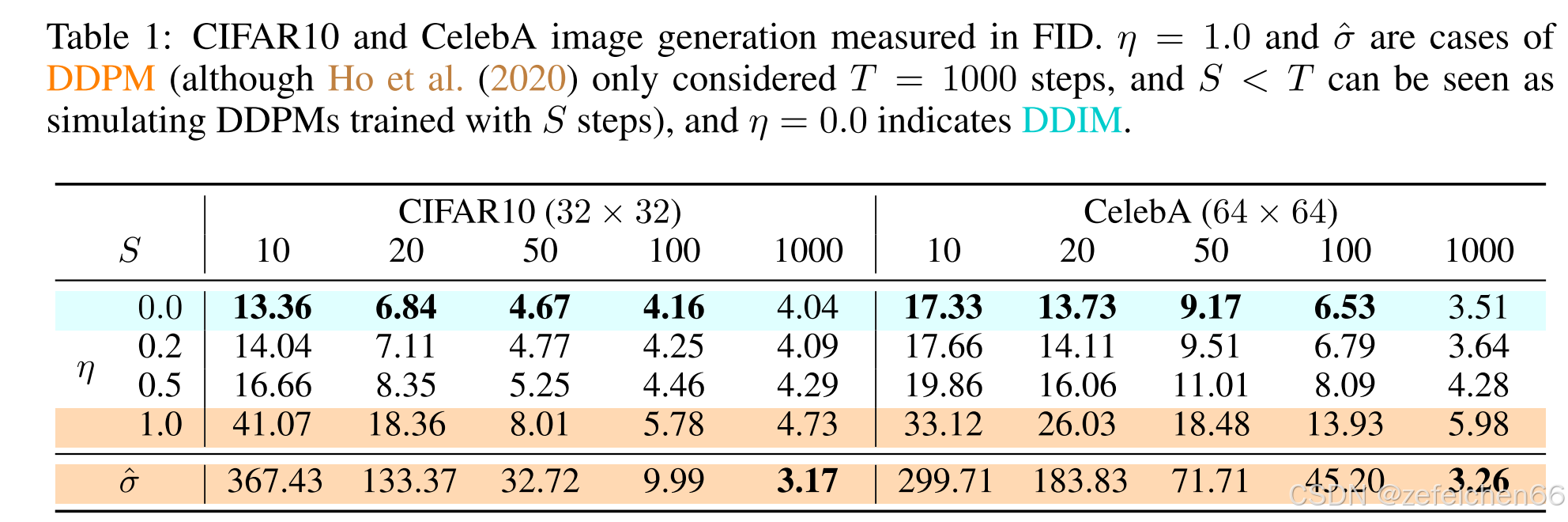
论文讨论了 σ t 2 \sigma_t^2 σt2选取 η ⋅ 1 − α t − 1 1 − α t ⋅ ( 1 − α t α t − 1 ) , η ∈ [ 0 , 1 ] \eta\cdot \frac{1-\alpha_{t-1}}{1-\alpha_t}\cdot (1-\frac{\alpha_t}{\alpha_{t-1}}),\eta\in[0,1] η⋅1−αt1−αt−1⋅(1−αt−1αt),η∈[0,1],即在0和DDPM之间变化时。不同 η \eta η以及跳不同步时所对应的表现,如下图所示。
5、代码
class DDIMPipeline(DiffusionPipeline):model_cpu_offload_seq = "unet"def __init__(self, unet, scheduler):super().__init__()# make sure scheduler can always be converted to DDIMscheduler = DDIMScheduler.from_config(scheduler.config)self.register_modules(unet=unet, scheduler=scheduler)@torch.no_grad()def __call__(self,batch_size: int = 1,generator: Optional[Union[torch.Generator, List[torch.Generator]]] = None,eta: float = 0.0,num_inference_steps: int = 50,use_clipped_model_output: Optional[bool] = None,output_type: Optional[str] = "pil",return_dict: bool = True,) -> Union[ImagePipelineOutput, Tuple]:# Sample gaussian noise to begin loopif isinstance(self.unet.config.sample_size, int):image_shape = (batch_size,self.unet.config.in_channels,self.unet.config.sample_size,self.unet.config.sample_size,)else:image_shape = (batch_size, self.unet.config.in_channels, *self.unet.config.sample_size)if isinstance(generator, list) and len(generator) != batch_size:raise ValueError(f"You have passed a list of generators of length {len(generator)}, but requested an effective batch"f" size of {batch_size}. Make sure the batch size matches the length of the generators.")# 随即生成噪音image = randn_tensor(image_shape, generator=generator, device=self._execution_device, dtype=self.unet.dtype)# 设置步数间隔。例如num_inference_steps = 50,然而总步长为1000,那么就是每次跳20步,例如在当前时刻, timestep=980, prev_timestep=960self.scheduler.set_timesteps(num_inference_steps)for t in self.progress_bar(self.scheduler.timesteps):# 1. 预测出timestep=980时刻对应噪音model_output = self.unet(image, t).sample# 2. 调用scheduler的方法step,执行公式()得到prev_timestep=960时刻的图像image = self.scheduler.step(model_output, t, image, eta=eta, use_clipped_model_output=use_clipped_model_output, generator=generator).prev_sampleimage = (image / 2 + 0.5).clamp(0, 1)image = image.cpu().permute(0, 2, 3, 1).numpy()if output_type == "pil":image = self.numpy_to_pil(image)if not return_dict:return (image,)return ImagePipelineOutput(images=image)class DDIMScheduler(SchedulerMixin, ConfigMixin):_compatibles = [e.name for e in KarrasDiffusionSchedulers]order = 1@register_to_configdef __init__(self,num_train_timesteps: int = 1000,beta_start: float = 0.0001,beta_end: float = 0.02,beta_schedule: str = "linear",trained_betas: Optional[Union[np.ndarray, List[float]]] = None,clip_sample: bool = True,set_alpha_to_one: bool = True,steps_offset: int = 0,prediction_type: str = "epsilon",thresholding: bool = False,dynamic_thresholding_ratio: float = 0.995,clip_sample_range: float = 1.0,sample_max_value: float = 1.0,timestep_spacing: str = "leading",rescale_betas_zero_snr: bool = False,):if trained_betas is not None:self.betas = torch.tensor(trained_betas, dtype=torch.float32)elif beta_schedule == "linear":self.betas = torch.linspace(beta_start, beta_end, num_train_timesteps, dtype=torch.float32)elif beta_schedule == "scaled_linear":# this schedule is very specific to the latent diffusion model.self.betas = torch.linspace(beta_start**0.5, beta_end**0.5, num_train_timesteps, dtype=torch.float32) ** 2elif beta_schedule == "squaredcos_cap_v2":# Glide cosine scheduleself.betas = betas_for_alpha_bar(num_train_timesteps)else:raise NotImplementedError(f"{beta_schedule} is not implemented for {self.__class__}")# Rescale for zero SNRif rescale_betas_zero_snr:self.betas = rescale_zero_terminal_snr(self.betas)self.alphas = 1.0 - self.betasself.alphas_cumprod = torch.cumprod(self.alphas, dim=0)# At every step in ddim, we are looking into the previous alphas_cumprod# For the final step, there is no previous alphas_cumprod because we are already at 0# `set_alpha_to_one` decides whether we set this parameter simply to one or# whether we use the final alpha of the "non-previous" one.self.final_alpha_cumprod = torch.tensor(1.0) if set_alpha_to_one else self.alphas_cumprod[0]# standard deviation of the initial noise distributionself.init_noise_sigma = 1.0# setable valuesself.num_inference_steps = Noneself.timesteps = torch.from_numpy(np.arange(0, num_train_timesteps)[::-1].copy().astype(np.int64))def scale_model_input(self, sample: torch.Tensor, timestep: Optional[int] = None) -> torch.Tensor:"""Ensures interchangeability with schedulers that need to scale the denoising model input depending on thecurrent timestep.Args:sample (`torch.Tensor`):The input sample.timestep (`int`, *optional*):The current timestep in the diffusion chain.Returns:`torch.Tensor`:A scaled input sample."""return sampledef _get_variance(self, timestep, prev_timestep):alpha_prod_t = self.alphas_cumprod[timestep]alpha_prod_t_prev = self.alphas_cumprod[prev_timestep] if prev_timestep >= 0 else self.final_alpha_cumprodbeta_prod_t = 1 - alpha_prod_tbeta_prod_t_prev = 1 - alpha_prod_t_prevvariance = (beta_prod_t_prev / beta_prod_t) * (1 - alpha_prod_t / alpha_prod_t_prev)return variance# Copied from diffusers.schedulers.scheduling_ddpm.DDPMScheduler._threshold_sampledef _threshold_sample(self, sample: torch.Tensor) -> torch.Tensor:""""Dynamic thresholding: At each sampling step we set s to a certain percentile absolute pixel value in xt0 (theprediction of x_0 at timestep t), and if s > 1, then we threshold xt0 to the range [-s, s] and then divide bys. Dynamic thresholding pushes saturated pixels (those near -1 and 1) inwards, thereby actively preventingpixels from saturation at each step. We find that dynamic thresholding results in significantly betterphotorealism as well as better image-text alignment, especially when using very large guidance weights."https://arxiv.org/abs/2205.11487"""dtype = sample.dtypebatch_size, channels, *remaining_dims = sample.shapeif dtype not in (torch.float32, torch.float64):sample = sample.float() # upcast for quantile calculation, and clamp not implemented for cpu half# Flatten sample for doing quantile calculation along each imagesample = sample.reshape(batch_size, channels * np.prod(remaining_dims))abs_sample = sample.abs() # "a certain percentile absolute pixel value"s = torch.quantile(abs_sample, self.config.dynamic_thresholding_ratio, dim=1)s = torch.clamp(s, min=1, max=self.config.sample_max_value) # When clamped to min=1, equivalent to standard clipping to [-1, 1]s = s.unsqueeze(1) # (batch_size, 1) because clamp will broadcast along dim=0sample = torch.clamp(sample, -s, s) / s # "we threshold xt0 to the range [-s, s] and then divide by s"sample = sample.reshape(batch_size, channels, *remaining_dims)sample = sample.to(dtype)return sampledef set_timesteps(self, num_inference_steps: int, device: Union[str, torch.device] = None):"""Sets the discrete timesteps used for the diffusion chain (to be run before inference).Args:num_inference_steps (`int`):The number of diffusion steps used when generating samples with a pre-trained model."""if num_inference_steps > self.config.num_train_timesteps:raise ValueError(f"`num_inference_steps`: {num_inference_steps} cannot be larger than `self.config.train_timesteps`:"f" {self.config.num_train_timesteps} as the unet model trained with this scheduler can only handle"f" maximal {self.config.num_train_timesteps} timesteps.")self.num_inference_steps = num_inference_steps# "linspace", "leading", "trailing" corresponds to annotation of Table 2. of https://arxiv.org/abs/2305.08891if self.config.timestep_spacing == "linspace":timesteps = (np.linspace(0, self.config.num_train_timesteps - 1, num_inference_steps).round()[::-1].copy().astype(np.int64))elif self.config.timestep_spacing == "leading":step_ratio = self.config.num_train_timesteps // self.num_inference_steps# creates integer timesteps by multiplying by ratio# casting to int to avoid issues when num_inference_step is power of 3timesteps = (np.arange(0, num_inference_steps) * step_ratio).round()[::-1].copy().astype(np.int64)timesteps += self.config.steps_offsetelif self.config.timestep_spacing == "trailing":step_ratio = self.config.num_train_timesteps / self.num_inference_steps# creates integer timesteps by multiplying by ratio# casting to int to avoid issues when num_inference_step is power of 3timesteps = np.round(np.arange(self.config.num_train_timesteps, 0, -step_ratio)).astype(np.int64)timesteps -= 1else:raise ValueError(f"{self.config.timestep_spacing} is not supported. Please make sure to choose one of 'leading' or 'trailing'.")self.timesteps = torch.from_numpy(timesteps).to(device)def step(self,model_output: torch.Tensor,timestep: int,sample: torch.Tensor,eta: float = 0.0,use_clipped_model_output: bool = False,generator=None,variance_noise: Optional[torch.Tensor] = None,return_dict: bool = True,) -> Union[DDIMSchedulerOutput, Tuple]:if self.num_inference_steps is None:raise ValueError("Number of inference steps is 'None', you need to run 'set_timesteps' after creating the scheduler")# 1. get previous step value (=t-1);# timestep=980,self.config.num_train_timesteps=1000, self.num_inference_steps=50# prev_timestep = 960,步数的跳跃间隔为20prev_timestep = timestep - self.config.num_train_timesteps // self.num_inference_steps# 2. compute alphas, betasalpha_prod_t = self.alphas_cumprod[timestep]alpha_prod_t_prev = self.alphas_cumprod[prev_timestep] if prev_timestep >= 0 else self.final_alpha_cumprodbeta_prod_t = 1 - alpha_prod_t# 3. compute predicted original sample from predicted noise also called# "predicted x_0" of formula (12) from https://arxiv.org/pdf/2010.02502.pdfif self.config.prediction_type == "epsilon":pred_original_sample = (sample - beta_prod_t ** (0.5) * model_output) / alpha_prod_t ** (0.5)pred_epsilon = model_outputelif self.config.prediction_type == "sample":pred_original_sample = model_outputpred_epsilon = (sample - alpha_prod_t ** (0.5) * pred_original_sample) / beta_prod_t ** (0.5)elif self.config.prediction_type == "v_prediction":pred_original_sample = (alpha_prod_t**0.5) * sample - (beta_prod_t**0.5) * model_outputpred_epsilon = (alpha_prod_t**0.5) * model_output + (beta_prod_t**0.5) * sampleelse:raise ValueError(f"prediction_type given as {self.config.prediction_type} must be one of `epsilon`, `sample`, or"" `v_prediction`")# 4. Clip or threshold "predicted x_0"if self.config.thresholding:pred_original_sample = self._threshold_sample(pred_original_sample)elif self.config.clip_sample:pred_original_sample = pred_original_sample.clamp(-self.config.clip_sample_range, self.config.clip_sample_range)# 5. compute variance: "sigma_t(η)" -> see formula (16)# σ_t = sqrt((1 − α_t−1)/(1 − α_t)) * sqrt(1 − α_t/α_t−1)variance = self._get_variance(timestep, prev_timestep)std_dev_t = eta * variance ** (0.5)if use_clipped_model_output:# the pred_epsilon is always re-derived from the clipped x_0 in Glidepred_epsilon = (sample - alpha_prod_t ** (0.5) * pred_original_sample) / beta_prod_t ** (0.5)# 6. compute "direction pointing to x_t" of formula (12) from https://arxiv.org/pdf/2010.02502.pdfpred_sample_direction = (1 - alpha_prod_t_prev - std_dev_t**2) ** (0.5) * pred_epsilon# 7. compute x_t without "random noise" of formula (12) from https://arxiv.org/pdf/2010.02502.pdfprev_sample = alpha_prod_t_prev ** (0.5) * pred_original_sample + pred_sample_directionif eta > 0:if variance_noise is not None and generator is not None:raise ValueError("Cannot pass both generator and variance_noise. Please make sure that either `generator` or"" `variance_noise` stays `None`.")if variance_noise is None:variance_noise = randn_tensor(model_output.shape, generator=generator, device=model_output.device, dtype=model_output.dtype)variance = std_dev_t * variance_noiseprev_sample = prev_sample + varianceif not return_dict:return (prev_sample,pred_original_sample,)return DDIMSchedulerOutput(prev_sample=prev_sample, pred_original_sample=pred_original_sample)# Copied from diffusers.schedulers.scheduling_ddpm.DDPMScheduler.add_noisedef add_noise(self,original_samples: torch.Tensor,noise: torch.Tensor,timesteps: torch.IntTensor,) -> torch.Tensor:# Make sure alphas_cumprod and timestep have same device and dtype as original_samples# Move the self.alphas_cumprod to device to avoid redundant CPU to GPU data movement# for the subsequent add_noise callsself.alphas_cumprod = self.alphas_cumprod.to(device=original_samples.device)alphas_cumprod = self.alphas_cumprod.to(dtype=original_samples.dtype)timesteps = timesteps.to(original_samples.device)sqrt_alpha_prod = alphas_cumprod[timesteps] ** 0.5sqrt_alpha_prod = sqrt_alpha_prod.flatten()while len(sqrt_alpha_prod.shape) < len(original_samples.shape):sqrt_alpha_prod = sqrt_alpha_prod.unsqueeze(-1)sqrt_one_minus_alpha_prod = (1 - alphas_cumprod[timesteps]) ** 0.5sqrt_one_minus_alpha_prod = sqrt_one_minus_alpha_prod.flatten()while len(sqrt_one_minus_alpha_prod.shape) < len(original_samples.shape):sqrt_one_minus_alpha_prod = sqrt_one_minus_alpha_prod.unsqueeze(-1)noisy_samples = sqrt_alpha_prod * original_samples + sqrt_one_minus_alpha_prod * noisereturn noisy_samples# Copied from diffusers.schedulers.scheduling_ddpm.DDPMScheduler.get_velocitydef get_velocity(self, sample: torch.Tensor, noise: torch.Tensor, timesteps: torch.IntTensor) -> torch.Tensor:# Make sure alphas_cumprod and timestep have same device and dtype as sampleself.alphas_cumprod = self.alphas_cumprod.to(device=sample.device)alphas_cumprod = self.alphas_cumprod.to(dtype=sample.dtype)timesteps = timesteps.to(sample.device)sqrt_alpha_prod = alphas_cumprod[timesteps] ** 0.5sqrt_alpha_prod = sqrt_alpha_prod.flatten()while len(sqrt_alpha_prod.shape) < len(sample.shape):sqrt_alpha_prod = sqrt_alpha_prod.unsqueeze(-1)sqrt_one_minus_alpha_prod = (1 - alphas_cumprod[timesteps]) ** 0.5sqrt_one_minus_alpha_prod = sqrt_one_minus_alpha_prod.flatten()while len(sqrt_one_minus_alpha_prod.shape) < len(sample.shape):sqrt_one_minus_alpha_prod = sqrt_one_minus_alpha_prod.unsqueeze(-1)velocity = sqrt_alpha_prod * noise - sqrt_one_minus_alpha_prod * samplereturn velocitydef __len__(self):return self.config.num_train_timesteps
相关文章:
)
论文阅读笔记:Denoising Diffusion Implicit Models (4)
0、快速访问 论文阅读笔记:Denoising Diffusion Implicit Models (1) 论文阅读笔记:Denoising Diffusion Implicit Models (2) 论文阅读笔记:Denoising Diffusion Implicit Models (…...

红帽Linux怎么重置密码
完整流程 ●重启操作系统,进入启动界面 ●然后按进入选择项界面 ●找到linux单词开头的那一行,然后移动到该行末尾(方向键移动或者使用键盘上的end),在末尾加入rd.break ●按ctrl x进入rd.break模式 ●在该模式下依次…...

关于存储的笔记
存储简介 名称适用场景常见运用网络环境备注块存储高性能、低延迟数据库局域网专业文件存储数据共享共享文件夹、非结构化数据局域网通用对象存储大数据、云存储网盘、网络媒体公网(断点续传、去重)海量 存储协议 名称协议块存储FC-SAN或IP-SAN承载的…...

java根据集合中对象的属性值大小生成排名
1:根据对象属性降序排列 public static <T extends Comparable<? super T>> LinkedHashMap<T, Integer> calculateRanking(List<ProductPerformanceInfoVO> dataList, Function<ProductPerformanceInfoVO, T> keyExtractor) {Linked…...

蓝桥杯嵌入式16届—— LED模块
使用主板 是STMG431RBT6 STMG431RBT6资源 资源配置表 跳线说明表 引脚状况 PC8~PC15分别对应着LD1~LD8 SN74HC573ADWR 是一种锁存器 当 LE(锁存使能)为高电平,输出 Q 实时跟随输入 D 的变化。当 LE 为低电平,输出锁定为最后…...

【IOS webview】源代码映射错误,页面卡住不动
报错场景 safari页面报源代码映射错误,页面卡住不动。 机型:IOS13 技术栈:react 其他IOS也会报错,但不影响页面显示。 debug webpack配置不要GENERATE_SOURCEMAP。 解决方法: GENERATE_SOURCEMAPfalse react-app…...

206. 反转链表 92. 反转链表 II 25. K 个一组翻转链表
leetcode Hot 100系列 文章目录 一、翻转链表二、反转链表 II三、K 个一组翻转链表总结 一、翻转链表 建立pre为空,建立cur为head,开始循环:先保存cur的next的值,再将cur的next置为pre,将pre前进到cur的位置…...
)
绘制动态甘特图(以流水车间调度为例)
import matplotlib.pyplot as plt import matplotlib.animation as animation import numpy as np from matplotlib import cm# 中文字体配置(必须放在所有绘图语句之前) plt.rcParams[font.sans-serif] [SimHei] plt.rcParams[axes.unicode_minus] Fa…...

生成式AI应用带来持续升级的网络安全风险
生成式AI应用带来持续升级的网络安全风险概要 根据Netskope最新研究,企业向生成式AI(GenAI)应用共享的数据量呈现爆炸式增长,一年内激增30倍。目前平均每家企业每月向AI工具传输的数据量已达7.7GB,较一年前的250MB实现…...

C++17更新内容汇总
C17 是 C14 的进一步改进版本,它引入了许多增强特性,优化了语法,并提升了编译期计算能力。以下是 C17 的主要更新内容: 1. 结构化绑定(Structured Bindings) 允许同时解构多个变量,从 std::tup…...

conda activate激活环境失败问题
出现 CondaError: Run conda init before conda activate 的错误,通常是因为 Conda 没有正确初始化当前的命令行环境。以下是解决方法: 1. 初始化 Conda 运行以下命令以初始化 Conda: conda init解释: conda init 会修改当前 S…...

TensorFlow实现逻辑回归
目录 前言TensorFlow实现逻辑回归 前言 实现逻辑回归的套路和实现线性回归差不多, 只不过逻辑回归的目标函数和损失函数不一样而已. TensorFlow实现逻辑回归 import tensorflow as tf import numpy as np import matplotlib.pyplot as plt from sklearn.datasets import mak…...

第十四届蓝桥杯大赛软件赛省赛Python 大学 C 组:6.棋盘
题目1 棋盘 小蓝拥有 nn 大小的棋盘,一开始棋盘上全都是白子。 小蓝进行了 m 次操作,每次操作会将棋盘上某个范围内的所有棋子的颜色取反(也就是白色棋子变为黑色,黑色棋子变为白色)。 请输出所有操作做完后棋盘上每个棋子的颜色。 输入格…...

电商场景下高稳定性数据接口的选型与实践
在电商系统开发中,API接口需要应对高并发请求、动态数据更新和复杂业务场景。我将重点解析电商场景对数据接口的特殊需求及选型方案。 一、电商API必备的四大核心能力 千万级商品数据实时同步 支持SKU基础信息/价格/库存多维度更新每日增量数据抓取与历史版本对比…...

内网服务器centos7安装jdk17
1. 下载 JDK 17 安装包(在外网环境操作) 在可联网的机器上下载 JDK 17 的压缩包(推荐使用 OpenJDK): OpenJDK 官方源: Adoptium Eclipse Temurin Azul Zulu 直接下载命令示例(在外网机器上执行…...

Git 使用教程
Git 使用教程 Git 是目前最流行的分布式版本控制系统,它能够高效地管理代码,并支持团队协作开发。本文将介绍 Git 的基本概念、常用命令以及如何在实际项目中使用 Git 进行版本控制。 1. Git 基本概念 在使用 Git 之前,需要了解以下几个基…...

【无标题】跨网段耦合器解决欧姆龙CJ系列PLC通讯问题案例
欧姆龙CJ系列PLC不同网段的通讯问题 一、项目背景 某大型制造企业的生产车间内,采用了多台欧姆龙CJ系列PLC对生产设备进行控制。随着企业智能化改造的推进,需要将这些PLC接入工厂的工业以太网,以便实现生产数据的实时采集、远程监控以及与企业…...

13_pandas可视化_seaborn
导入库 import numpy as np import pandas as pd # import matplotlib.pyplot as plt #交互环境中不需要导入 import seaborn as sns sns.set_context({figure.figsize:[8, 6]}) # 设置图大小 # 屏蔽警告 import warnings warnings.filterwarnings("ignore")关系图 …...

【C++进阶四】vector模拟实现
目录 1.构造函数 (1)无参构造 (2)带参构造函数 (3)用迭代器构造初始化函数 (4)拷贝构造函数 2.operator= 3.operator[] 4.size() 5.capacity() 6.push_back 7.reserve 8.迭代器(vector的原生指针) 9.resize 10.pop_back 11.insert 12.erase 13.memcpy…...
)
14使用按钮实现helloworld(1)
目录 还可以通过按钮的方式来创建 hello world 涉及Qt 中的信号槽机制本质就是给按钮的点击操作,关联上一个处理函数当用户点击的时候 就会执行这个处理函数 connect(谁发的信号, 信号类型, 谁来处理这个信息, 怎么处理的&…...

嵌入式EMC设计面试题及参考答案
目录 解释 EMC(电磁兼容性)的定义及其两个核心方面(EMI 和 EMS) 电磁兼容三要素及相互关系 为什么产品必须进行 EMC 设计?列举至少三个实际工程原因 分贝(dB)在 EMC 测试中的作用是什么?为何采用对数单位描述干扰强度? 传导干扰与辐射干扰的本质区别及典型频率范围…...

cursor的.cursorrules详解
文章目录 1. 文件位置与作用2. 基本语法规则3. 常用规则类型与示例3.1 忽略文件/目录3.2 限制代码生成范围3.3 自定义补全建议3.4 安全规则 4. 高级用法4.1 条件规则4.2 正则表达式匹配4.3 继承规则 5. 示例文件6. 注意事项 Cursor 是一款基于 AI 的智能代码编辑器,…...

Opencv计算机视觉编程攻略-第七节 提取直线、轮廓和区域
第七节 提取直线、轮廓和区域 1.用Canny 算子检测图像轮廓2.用霍夫变换检测直线;3.点集的直线拟合4.提取连续区域5.计算区域的形状描述子 图像的边缘区域勾画出了图像含有重要的视觉信息。正因如此,边缘可应用于目标识别等领域。但是简单的二值边缘分布图…...

清明假期在即
2025年4月2日,6~22℃,一般 遇见的事:这么都是清明出去玩?你们不扫墓的么。 感受到的情绪:当精力不放在一个人身上,你就会看到很多人,其实可以去接触的。 反思:抖音上那么多不幸和幸…...

数字孪生技术解析:开启虚拟与现实融合新时代
一、数字孪生技术的概念与原理 数字孪生技术是一种通过构建物理对象的数字映射,实现虚拟与现实同步的技术。该技术集成了物联网、云计算、人工智能、大数据等多种前沿技术,能够对物理世界进行全方位的仿真和管理。在数字孪生技术中,物理建模…...

Docker Registry 清理镜像最佳实践
文章目录 registry-clean1. 简介2. 功能3. 安装 docker4. 配置 docker5. 配置域名解析6. 部署 registry7. Registry API 管理8. 批量清理镜像9. 其他10. 参考 registry-clean 1. 简介 registry-clean 是一个强大而高效的解决方案,旨在简化您的 Docker 镜像仓库管理…...

进程间的通信
一.理解 1.进程间通信的目的 数据传输,资源共享,通知事件,进程控制 2.进程间通信的本质 先让不同的进程看到"同一份"资源(该资源只能由OS系统提供,不能由任何一个进程提供) 3.具体通信方式 …...

当实时消费遇到 SPL:让数据处理更高效、简单
作者:豁朗 通过 SPL 消费,将业务逻辑“左移” SLS 对实时消费进行了功能升级,推出了 基于 SPL 的规则消费功能。在实时消费过程中,用户只需通过简单的 SPL 配置即可完成服务端的数据清洗和预处理操作。通过SPL消费可以将客户端复…...
)
Python----机器学习(线性回归:反向传播和梯度下降)
一、前向传播与反向传播的区别 前向传播是在参数固定后,向公式中传入参数,进行预测的一个过程。当参 数值选择的不恰当时,会导致最后的预测值不符合我们的预期,于是我们就 需要重新修改参数值。 在前向传播实验中时,我…...

如何平衡元器件成本与性能
要平衡元器件成本与性能,企业应当明确设计需求和目标、优化元器件选型策略、建立成本性能评估体系、推进标准化设计、加强供应链管理。其中,优化元器件选型策略尤其关键,它直接关系到产品的成本、性能与生命周期。在选型时,工程师…...

java项目分享-分布式电商项目附软件链接
今天来分享一下github上最热门的开源电商项目安装部署,star 12.2k,自行安装部署历时两天,看了这篇文章快的话半天搞定!该踩的坑都踩完了,软件也打包好了就差喂嘴里。 项目简介 mall-swarm是一套微服务商城系统…...

低代码框架
在数字化转型浪潮中,软件开发的效率与成本成为企业关注的焦点。低代码框架应运而生,以其独特的开发模式,打破了传统软件开发的壁垒,为企业和开发者带来了全新的解决方案。那么,究竟什么是低代码框架呢? …...

Git Reset 命令详解与实用示例
文章目录 Git Reset 命令详解与实用示例git reset 主要选项git reset 示例1. 撤销最近一次提交(但保留更改)2. 撤销最近一次提交,并清除暂存区3. 彻底撤销提交,并丢弃所有更改4. 回退到特定的提交5. 取消暂存的文件 git reset 与 …...
)
多层内网渗透测试虚拟仿真实验环境(Tomcat、ladon64、frp、Weblogic、权限维持、SSH Server Wrapper后门)
在线环境:https://www.yijinglab.com/ 拓扑图 信息收集 IP地址扫描 确定目标IP为10.1.1.121 全端口扫描 访问靶机8080端口,发现目标是一个Tomcat服务,版本...

<贪心算法>
前言:在主包还没有接触算法的时候,就常听人提起“贪心”,当时是layman,根本不知道说的是什么,以为很难呢,但去了解一下,发现也不过如此嘛(bushi),还以为是什么高级东西呢…...
并训练Fashion-MNIST)
使用PyTorch实现GoogleNet(Inception)并训练Fashion-MNIST
GoogleNet(又称Inception v1)是2014年ILSVRC冠军模型,其核心创新是Inception模块,通过并行多尺度卷积提升特征提取能力。本文将展示如何用PyTorch实现GoogleNet,并在Fashion-MNIST数据集上进行训练。 1. 环境准备 im…...

KingbaseES物理备份还原之备份还原
此篇续接上一篇<<KingbaseES物理备份还原之物理备份>>,上一篇写物理备份相关操作,此篇写备份还原的具体操作步骤. KingbaseES版本:V009R004C011B003 一.执行最新物理备份还原 --停止数据库服务,并创建物理备份还原测试目录 [V9R4C11B3192-168-198-198 V8]$ sys_ct…...
之ForwardAdd(标准版))
Unity Standard Shader 解析(二)之ForwardAdd(标准版)
一、ForwardAdd // Additive forward pass (one light per pass)Pass{Name "FORWARD_DELTA"Tags { "LightMode" "ForwardAdd" }Blend [_SrcBlend] OneFog { Color (0,0,0,0) } // in additive pass fog should be blackZWrite OffZTest LEqual…...

.NET 使用 WMQ 连接Queue 发送 message 实例
1. 首先得下载客户端,没有客户端无法发送message. 安装好之后长这样 我装的是7.5 安装目录如下 tools/dotnet 目录中有演示的demo 2. .Net 连接MQ必须引用bin目录中的 amqmdnet.dll 因为他是创建Queuemanager 的核心库, 项目中引用using IBM.WMQ; 才…...

设计模式之单例模式
视频链接: 设计模式|狂神说 单例模式是什么? 单例模式是确保一个类在整个应用程序中只有一个实例,并提供一个全局方法访问这个实例。 单例模式分为饿汉式和懒汉式。 饿汉式单例 饿汉式顾名思义就是,程序一启动就创建这个单例bea…...

从入门到入土,SQLServer 2022慢查询问题总结
列为,由于公司原因,作者接触了一个SQLServer 2022作为数据存储到项目,可能是上一任的哥们儿离开的时候带有情绪,所以现在项目的主要问题就是,所有功能都实现了,但是就是慢,列表页3s打底,客户很生气,经过几周摸爬滚打,作以下总结,作为自己的成长记录。 一、索引问题…...

大语言模型在端到端智驾中的应用
大语言模型在端到端智驾中的应用 双系统端到端 小鹏:AI天玑系统—神经网络XNet规控大模型XPlanner大语言模型XBrain 商汤绝影:DriveAGI 理想:端到端VLM VLA端到端 Waymo:EMMA OPENEMMA Wayve:LINGO-2...
——基于miniQMT的量化交易回测系统开发实记)
【深度学习量化交易19】行情数据获取方式比测(1)——基于miniQMT的量化交易回测系统开发实记
我是Mr.看海,我在尝试用信号处理的知识积累和思考方式做量化交易,应用深度学习和AI实现股票自动交易,目的是实现财务自由~ 目前我正在开发基于miniQMT的量化交易系统——看海量化交易系统。 经常使用MiniQMT的朋友都知道,xtquant的…...

《网络管理》实践环节03:snmp服务器上对网络设备和服务器进行初步监控
兰生幽谷,不为莫服而不芳; 君子行义,不为莫知而止休。 应用拓扑图 3.0准备工作 所有Linux服务器上(服务器和Agent端)安装下列工具 yum -y install net-snmp net-snmp-utils 保证所有的HCL网络设备和服务器相互间能…...

linux操作系统
1.linux进程管理 操作系统都有进程的概念 查看和关闭程序 2.关闭进程 3,查看计算机硬件信息 4.定时任务...

Python基础语法 - 判断语句
Python基础语法 - 判断语句 1. if语句 if 条件:# 条件为True时执行的代码示例 age 18 if age > 18:print("您已成年")2. if-else语句 if 条件:# 条件为True时执行的代码 else:# 条件为False时执行的代码示例 age 16 if age > 18:print("您已成年&q…...

c++柔性数组、友元、类模版
目录 1、柔性数组: 2、友元函数: 3、静态成员 注意事项 面试题:c/c static的作用? C语言: C: 为什么可以创建出 objx 4、对象与对象之间的关系 5、类模版 1、柔性数组: #define _CRT_SECURE_NO_WARNINGS #…...

电子技术基础
目录 一、整体概述 二、知识点梳理及考点分析 (一)半导体器件 (二)基本放大电路 (三)功率放大电路 (四)集成运算放大器 (五)直流稳压电源 ࿰…...

解码大模型时代算力基座的隐形引擎
在千亿参数大模型竞速的今天,算力军备竞赛已进入白热化阶段。当我们聚焦GPU集群的运算峰值时,一个关键命题正在浮出水面:支撑大模型全生命周期的存力基座,正在成为制约AI进化的关键变量。绿算技术将深入解剖大模型训练与推理场景中…...

【NetCore】ControllerBase:ASP.NET Core 中的基石类
ControllerBase:ASP.NET Core 中的基石类 一、什么是 ControllerBase?二、ControllerBase 的主要功能三、ControllerBase 的常用属性四、ControllerBase 的常用方法2. 模型绑定与验证3. 依赖注入五、ControllerBase 与 Controller 的区别六、实际开发中的最佳实践七、总结在 …...