当前位置：首页 > news >正文

经典NLP案例 | 推文评论情绪分析：从数据预处理到模型构建的全面指南

news 来源：原创 2025/6/25 11:38:20

NLP经典案例：推文评论情绪提取

项目背景

“My ridiculous dog is amazing.” [sentiment: positive]

由于所有推文每秒都在传播，很难判断特定推文背后的情绪是否会影响一家公司或一个人的品牌，因为它的病毒式传播（积极），或者因为它的负面基调而破坏利润。在决策和反应在几秒钟内创建和更新的时代，用语言捕捉情感非常重要。但是，哪些词实际上导致了情感描述呢？在本次比赛中，您需要选出推文中反映情绪的部分（单词或短语）。

利用这个广泛的推文数据集帮助您培养在这一重要领域的技能。努力提高你的技术，在这场比赛中占据榜首。推文中的哪些词语支持积极、消极或中立的情绪？您如何使用机器学习工具帮助做出决定？

在本次比赛中，我们从 Figure Eight 的 Data for Everyone 平台中提取了支持短语。该数据集的标题为“情感分析：具有现有情感标签的文本推文中的情感”，此处在知识共享署名 4.0 下使用。国际许可证。你在这次比赛中的目标是构建一个可以做同样事情的模型 - 查看给定推文的标记情绪，并找出最能支持它的单词或短语。

关于本项目

在此笔记中，我将简要解释数据集的结构。我将生成并分析元特征。然后，我将使用 Matplotlib、seaborn 和 Plotly 可视化数据集，以获得尽可能多的见解。我还将把这个问题作为 NER 问题来处理来构建模型

导入必要的库

import re
import string
import numpy as np 
import random
import pandas as pd 
import matplotlib.pyplot as plt
import seaborn as sns
%matplotlib inline
from plotly import graph_objs as go
import plotly.express as px
import plotly.figure_factory as ff
from collections import Counterfrom PIL import Image
from wordcloud import WordCloud, STOPWORDS, ImageColorGeneratorimport nltk
from nltk.corpus import stopwordsfrom tqdm import tqdm
import os
import nltk
import spacy
import random
from spacy.util import compounding
from spacy.util import minibatchimport warnings
warnings.filterwarnings("ignore")import os
for dirname, _, filenames in os.walk('/kaggle/input'):for filename in filenames:print(os.path.join(dirname, filename))# 您写入当前目录的任何结果都将保存为输出。

下面是一个辅助函数，它生成随机颜色，可用于为您的绘图提供不同的颜色。随意使用它

def random_colours(number_of_colors):'''随机颜色生成的简单函数。输入：number_of_colors -指示将生成的颜色数量的整数值。输出：采用以下格式的颜色： ['#E86DA4'] 。'''colors = []for i in range(number_of_colors):colors.append("#"+''.join([random.choice('0123456789ABCDEF') for j in range(6)]))return colors

读取数据

本项目数据集来源于kaggle竞赛平台，可公众号后台回复“推文情绪”即可获取数据集

train = pd.read_csv('/kaggle/input/tweet-sentiment-extraction/train.csv')
test = pd.read_csv('/kaggle/input/tweet-sentiment-extraction/test.csv')
ss = pd.read_csv('/kaggle/input/tweet-sentiment-extraction/sample_submission.csv')

print(train.shape)
print(test.shape)

(27481, 4)
(3534, 3)

所以我们在训练集中有 27486 条推文，在测试集中有 3535 条推文

train.info()

<class 'pandas.core.frame.DataFrame'>
RangeIndex: 27481 entries, 0 to 27480
Data columns (total 4 columns):
textID           27481 non-null object
text             27480 non-null object
selected_text    27480 non-null object
sentiment        27481 non-null object
dtypes: object(4)
memory usage: 858.9+ KB

我们在训练中有一个空值，因为值的测试字段是 NAN，我们将删除它

train.dropna(inplace=True)

test.info()

<class 'pandas.core.frame.DataFrame'>
RangeIndex: 3534 entries, 0 to 3533
Data columns (total 3 columns):
textID       3534 non-null object
text         3534 non-null object
sentiment    3534 non-null object
dtypes: object(3)
memory usage: 83.0+ KB

测试集中不存在空值

EDA（数据探索性分析）

train.head()

Selected_text 是文本的子集

train.describe()

让我们看看推文在训练集中的分布

temp = train.groupby('sentiment').count()['text'].reset_index().sort_values(by='text',ascending=False)
temp.style.background_gradient(cmap='Purples')

	sentiment	text
1	neutral	11117
2	positive	8582
0	negative	7781

plt.figure(figsize=(12,6))
sns.countplot(x='sentiment',data=train)

让我们画一个漏斗图以获得更好的可视化效果

fig = go.Figure(go.Funnelarea(text =temp.sentiment,values = temp.text,title = {"position": "top center", "text": "Funnel-Chart of Sentiment Distribution"}))
fig.show()

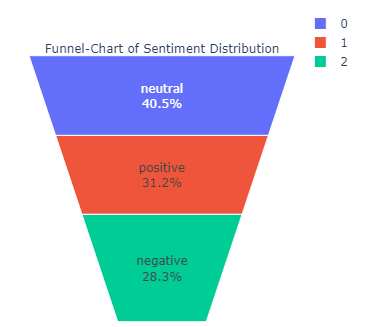
目前我们对数据了解多少：

在开始之前，让我们看一下我们已经了解的有关数据的一些知识，这些知识将帮助我们获得更多新的见解：

我们知道 selected_text 是文本的子集
我们知道 selected_text 只包含一段文本，即，它不会在两个句子之间跳转。例如：-如果文本是“在与供应商的会议中度过了整个上午，而我的老板对此不满意”他们。很有趣。我早上还有其他计划”所选文本可以是“我的老板对他们不满意”。很有趣”或“很有趣”，但不能是“早上好，供应商和我的老板，
我们知道中性推文的文本和 selected_text 之间的 jaccard 相似度为 97%
另外，有些行中 selected_text 从单词之间开始，因此 selected_texts 并不总是有意义，因为我们不知道是否测试集的输出是否包含这些差异，我们不确定预处理和删除标点符号是否是一个好主意

生成元特征

在本笔记本的先前版本中，我使用所选文本和主要文本中的单词数、文本中的单词长度和选择作为主要元特征，但在本次比赛的背景下，我们必须预测 selected_text 这是一个文本的子集，生成的更有用的功能将是：

Selected_text 和 Text 的字数差异
文本和 Selected_text 之间的 Jaccard 相似度分数

因此，生成我们之前使用过的特征对我们来说没有用，因为它们在这里并不重要

以下是 Jaccard 相似度的介绍：https://www.geeksforgeeks.org/find-the-jaccard-index-and-jaccard-distance-Between-the-two-given-sets/

def jaccard(str1, str2): a = set(str1.lower().split()) b = set(str2.lower().split())c = a.intersection(b)return float(len(c)) / (len(a) + len(b) - len(c))

results_jaccard=[]for ind,row in train.iterrows():sentence1 = row.textsentence2 = row.selected_textjaccard_score = jaccard(sentence1,sentence2)results_jaccard.append([sentence1,sentence2,jaccard_score])

jaccard = pd.DataFrame(results_jaccard,columns=["text","selected_text","jaccard_score"])
train = train.merge(jaccard,how='outer')

train['Num_words_ST'] = train['selected_text'].apply(lambda x:len(str(x).split())) #Number Of words in Selected Text
train['Num_word_text'] = train['text'].apply(lambda x:len(str(x).split())) #Number Of words in main text
train['difference_in_words'] = train['Num_word_text'] - train['Num_words_ST'] #Difference in Number of words text and Selected Text

train.head()

我们看一下Meta-Features的分布

hist_data = [train['Num_words_ST'],train['Num_word_text']]group_labels = ['Selected_Text', 'Text']# 使用自定义 bin_size 创建 distplot
fig = ff.create_distplot(hist_data, group_labels,show_curve=False)
fig.update_layout(title_text='Distribution of Number Of words')
fig.update_layout(autosize=False,width=900,height=700,paper_bgcolor="LightSteelBlue",
)
fig.show()

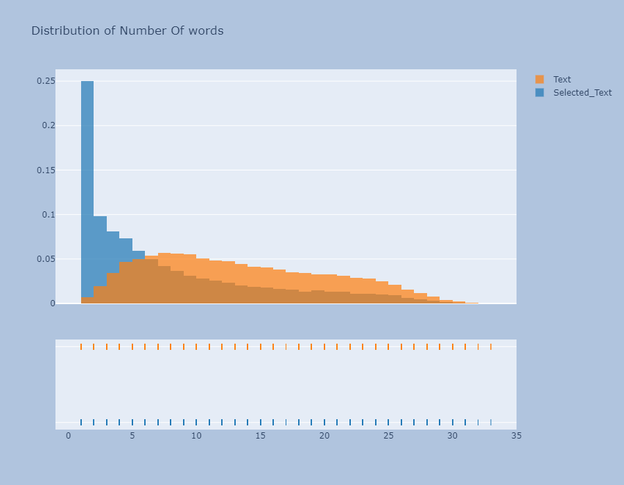
字数图非常有趣，字数大于 25 的推文非常少，因此字数分布图是右偏的

plt.figure(figsize=(12,6))
p1=sns.kdeplot(train['Num_words_ST'], shade=True, color="r").set_title('Kernel Distribution of Number Of words')
p1=sns.kdeplot(train['Num_word_text'], shade=True, color="b")

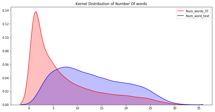
现在看到不同情绪的字数和jaccard分数的差异会更有趣

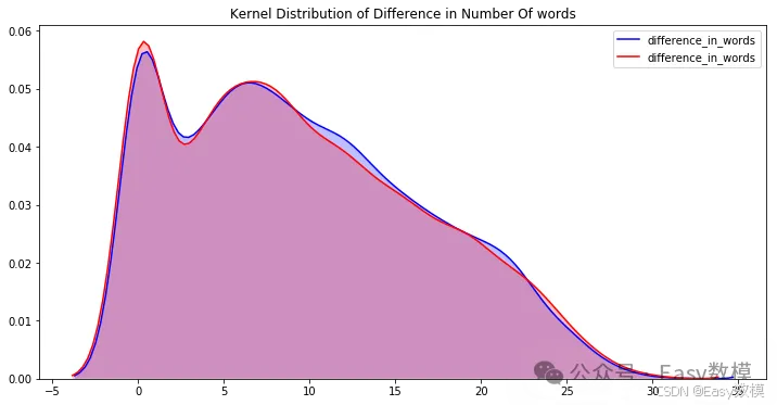
plt.figure(figsize=(12,6))
p1=sns.kdeplot(train[train['sentiment']=='positive']['difference_in_words'], shade=True, color="b").set_title('Kernel Distribution of Difference in Number Of words')
p2=sns.kdeplot(train[train['sentiment']=='negative']['difference_in_words'], shade=True, color="r")

在这里插入图片描述

plt.figure(figsize=(12,6))
sns.distplot(train[train['sentiment']=='neutral']['difference_in_words'],kde=False)

我无法绘制中性推文的 kde 图，因为大多数字数差异值为零。我们现在可以清楚地看到这一点，如果我们一开始就使用了该功能，我们就会知道对于中性推文来说，文本和所选文本大多相同，因此在执行 EDA 时牢记最终目标始终很重要

plt.figure(figsize=(12,6))
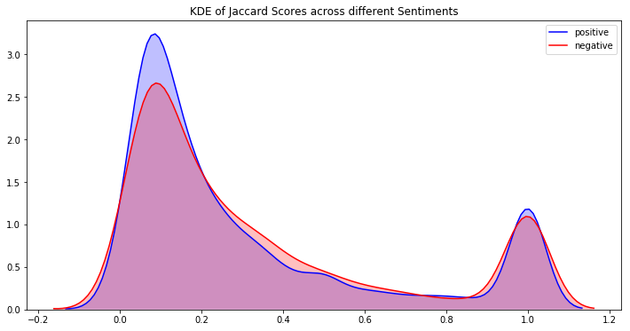
p1=sns.kdeplot(train[train['sentiment']=='positive']['jaccard_score'], shade=True, color="b").set_title('KDE of Jaccard Scores across different Sentiments')
p2=sns.kdeplot(train[train['sentiment']=='negative']['jaccard_score'], shade=True, color="r")
plt.legend(labels=['positive','negative'])

<matplotlib.legend.Legend at 0x7f99682eac50>

出于同样的原因，我无法绘制中立推文的 jaccard_scores 的 kde，因此我将绘制分布图

plt.figure(figsize=(12,6))
sns.distplot(train[train['sentiment']=='neutral']['jaccard_score'],kde=False)

我们可以在这里看到一些有趣的趋势：

正面和负面推文具有高峰度，因此值集中在窄和高密度两个区域
中性推文具有较低的峰度值，并且其密度波动接近 1

定义解释：

峰度是分布的峰值程度以及围绕该峰值的分布程度的度量
偏度衡量曲线偏离正态分布的程度

EDA结论

我们可以从 jaccard 分数图中看到，分数为 1 附近有负图和正图的峰值。这意味着存在一组推文，其中文本和所选文本之间存在高度相似性，如果我们可以找到这些聚类，那么我们可以预测这些推文的选定文本的文本，无论片段如何

让我们看看是否可以找到这些簇，一个有趣的想法是检查文本中单词数少于 3 个的推文，因为那里的文本可能完全用作文本

k = train[train['Num_word_text']<=2]

k.groupby('sentiment').mean()['jaccard_score']

sentiment
negative    0.788580
neutral     0.977805
positive    0.765700
Name: jaccard_score, dtype: float64

我们可以看到文本和所选文本之间存在相似性。让我们仔细看看

k[k['sentiment']=='positive']

因此很明显，大多数时候，文本被用作选定文本。我们可以通过预处理字长小于3的文本来改进这一点。我们将记住这些信息并在模型构建中使用它。

清理语料库

现在，在我们深入从文本和选定文本中的单词中提取信息之前，让我们首先清理数据。

def clean_text(text):'''将文本设为小写、删除方括号中的文本、删除链接、删除标点符号并删除包含数字的单词。'''text = str(text).lower()text = re.sub('\[.*?\]', '', text)text = re.sub('https?://\S+|www\.\S+', '', text)text = re.sub('<.*?>+', '', text)text = re.sub('[%s]' % re.escape(string.punctuation), '', text)text = re.sub('\n', '', text)text = re.sub('\w*\d\w*', '', text)return text

train['text'] = train['text'].apply(lambda x:clean_text(x))
train['selected_text'] = train['selected_text'].apply(lambda x:clean_text(x))

train.head()

我们的目标选定文本中最常见的单词

train['temp_list'] = train['selected_text'].apply(lambda x:str(x).split())
top = Counter([item for sublist in train['temp_list'] for item in sublist])
temp = pd.DataFrame(top.most_common(20))
temp.columns = ['Common_words','count']
temp.style.background_gradient(cmap='Blues')

Index	Common_words	count
0	i	7200
1	to	5305
2	the	4590
3	a	3538
4	my	2783
5	you	2624
6	and	2321
7	it	2158
8	is	2115
9	in	1986
10	for	1854
11	im	1676
12	of	1638
13	me	1540
14	on	1488
15	so	1410
16	have	1345
17	that	1297
18	but	1267
19	good	1251

fig = px.bar(temp, x="count", y="Common_words", title='Commmon Words in Selected Text', orientation='h', width=700, height=700,color='Common_words')
fig.show()

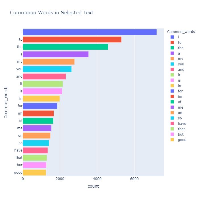
哎呀！当我们清理数据集时，我们没有删除停用词，因此我们可以看到最常见的词是 ‘to’ 。删除停用词后重试

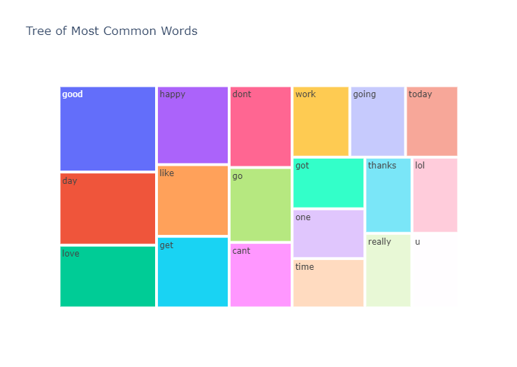
def remove_stopword(x):return [y for y in x if y not in stopwords.words('english')]
train['temp_list'] = train['temp_list'].apply(lambda x:remove_stopword(x))

top = Counter([item for sublist in train['temp_list'] for item in sublist])
temp = pd.DataFrame(top.most_common(20))
temp = temp.iloc[1:,:]
temp.columns = ['Common_words','count']
temp.style.background_gradient(cmap='Purples')

Index	Common_words	count
1	good	1251
2	day	1058
3	love	909
4	happy	852
5	like	774
6	get	772
7	dont	765
8	go	700
9	cant	613
10	work	612
11	going	592
12	today	564
13	got	558
14	one	538
15	time	534
16	thanks	532
17	lol	528
18	really	520
19	u	519

fig = px.treemap(temp, path=['Common_words'], values='count',title='Tree of Most Common Words')
fig.show()

文本中最常见的单词

我们还看一下 Text 中最常见的单词

train['temp_list1'] = train['text'].apply(lambda x:str(x).split()) #文本每行的单词列表
train['temp_list1'] = train['temp_list1'].apply(lambda x:remove_stopword(x)) #删除停用词

top = Counter([item for sublist in train['temp_list1'] for item in sublist])
temp = pd.DataFrame(top.most_common(25))
temp = temp.iloc[1:,:]
temp.columns = ['Common_words','count']
temp.style.background_gradient(cmap='Blues')

Index	Common_words	count
1	day	2044
2	good	1549
3	get	1426
4	like	1346
5	go	1267
6	dont	1200
7	love	1122
8	work	1112
9	going	1096
10	today	1096
11	got	1072
12	cant	1020
13	happy	976
14	one	971
15	lol	948
16	time	942
17	know	930
18	u	923
19	really	908
20	back	891
21	see	797
22	well	744
23	new	740
24	night	737

所以前两个常见词是我，所以我删除了它并从第二行获取数据

fig = px.bar(temp, x="count", y="Common_words", title='Commmon Words in Text', orientation='h', width=700, height=700,color='Common_words')
fig.show()

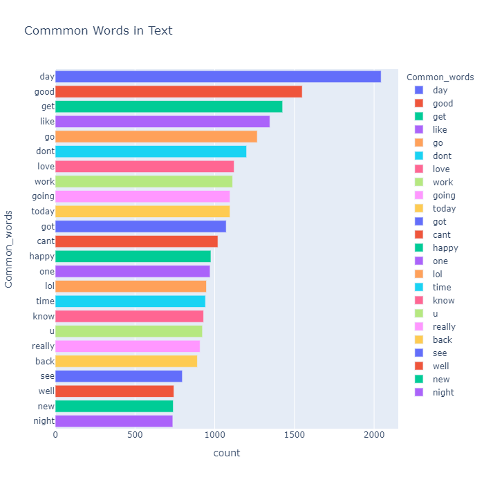
所以我们可以看到所选文本和文本中最常见的单词几乎相同，这是显而易见的

最常用的词情感明智

让我们看看不同情绪中最常见的单词

Positive_sent = train[train['sentiment']=='positive']
Negative_sent = train[train['sentiment']=='negative']
Neutral_sent = train[train['sentiment']=='neutral']

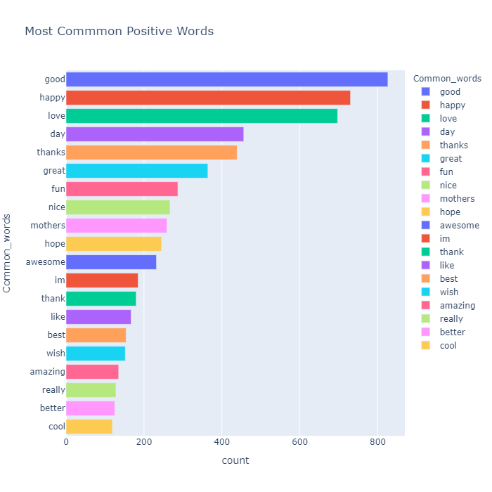
#最常见的正面词汇
top = Counter([item for sublist in Positive_sent['temp_list'] for item in sublist])
temp_positive = pd.DataFrame(top.most_common(20))
temp_positive.columns = ['Common_words','count']
temp_positive.style.background_gradient(cmap='Greens')

Index	Common_words	count
0	good	826
1	happy	730
2	love	697
3	day	456
4	thanks	439
5	great	364
6	fun	287
7	nice	267
8	mothers	259
9	hope	245
10	awesome	232
11	im	185
12	thank	180
13	like	167
14	best	154
15	wish	152
16	amazing	135
17	really	128
18	better	125
19	cool	119

fig = px.bar(temp_positive, x="count", y="Common_words", title='Most Commmon Positive Words', orientation='h', width=700, height=700,color='Common_words')
fig.show()

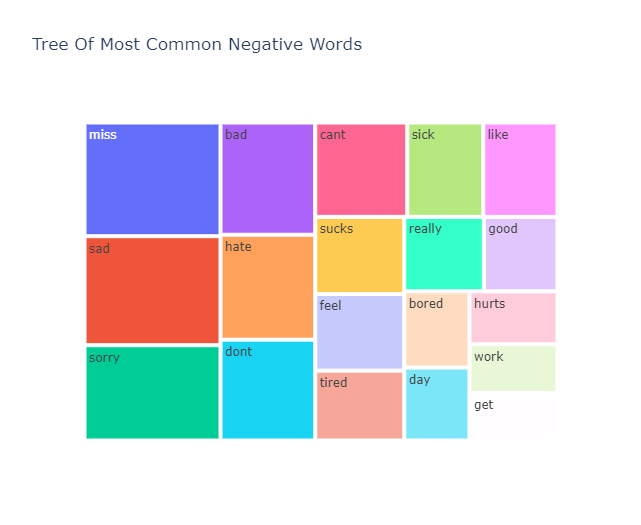
#最常见的负面词
top = Counter([item for sublist in Negative_sent['temp_list'] for item in sublist])
temp_negative = pd.DataFrame(top.most_common(20))
temp_negative = temp_negative.iloc[1:,:]
temp_negative.columns = ['Common_words','count']
temp_negative.style.background_gradient(cmap='Reds')

Index	Common_words	count
1	miss	358
2	sad	343
3	sorry	300
4	bad	246
5	hate	230
6	dont	221
7	cant	201
8	sick	166
9	like	162
10	sucks	159
11	feel	158
12	tired	144
13	really	137
14	good	127
15	bored	115
16	day	110
17	hurts	108
18	work	99
19	get	97

fig = px.treemap(temp_negative, path=['Common_words'], values='count',title='Tree Of Most Common Negative Words')
fig.show()

#最常见的中性词
top = Counter([item for sublist in Neutral_sent['temp_list'] for item in sublist])
temp_neutral = pd.DataFrame(top.most_common(20))
temp_neutral = temp_neutral.loc[1:,:]
temp_neutral.columns = ['Common_words','count']
temp_neutral.style.background_gradient(cmap='Reds')

Index	Common_words	count
1	get	612
2	go	569
3	day	492
4	dont	482
5	going	472
6	work	467
7	like	445
8	got	441
9	today	427
10	lol	427
11	time	413
12	know	407
13	back	402
14	one	394
15	u	376
16	see	349
17	cant	339
18	home	335
19	want	319

fig = px.bar(temp_neutral, x="count", y="Common_words", title='Most Commmon Neutral Words', orientation='h', width=700, height=700,color='Common_words')
fig.show()

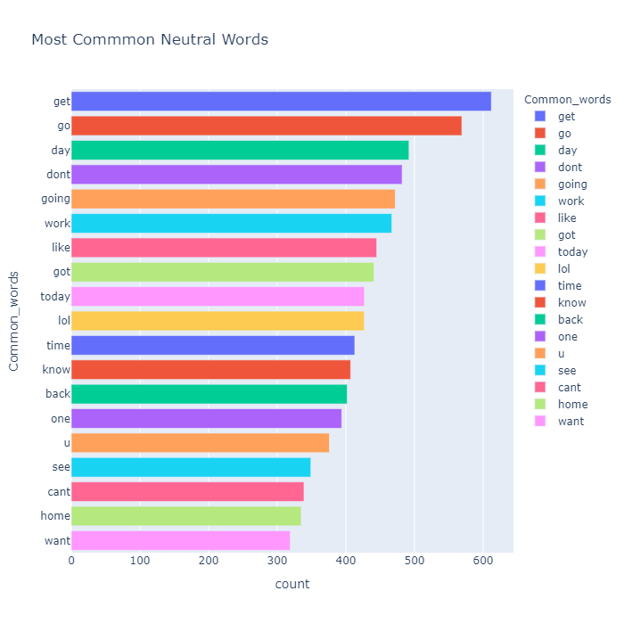
fig = px.treemap(temp_neutral, path=['Common_words'], values='count',title='Tree Of Most Common Neutral Words')
fig.show()

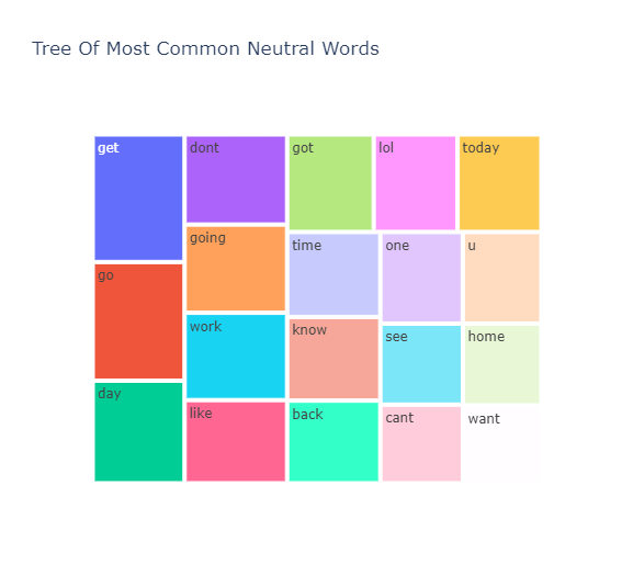
我们可以看到 get、go、dont、got、u、cant、lol、like 等词在这三个细分市场中都很常见。这很有趣，因为像 dont 和 cant 这样的词更多的是消极的性质，而像 lol 这样的词更多的是积极的性质。这是否意味着我们的数据被错误地标记了，在 N-gram 分析后我们将对此有更多的见解

看到不同情绪所特有的词会很有趣

让我们看看每个片段中的独特单词

我们将按以下顺序查看每个片段中的唯一单词：

积极的
消极的
中性的

raw_text = [word for word_list in train['temp_list1'] for word in word_list]

def words_unique(sentiment,numwords,raw_words):'''输入：细分 -细分类别（例如“中性”）；numwords -您希望在最终结果中看到多少个特定单词； raw_words -train_data[train_data.segments == snippets]['temp_list1'] 中的项目列表：输出： 数据框提供有关特定成分名称及其在所选菜肴中出现的次数的信息（根据其计数按降序排列）..'''allother = []for item in train[train.sentiment != sentiment]['temp_list1']:for word in item:allother .append(word)allother  = list(set(allother ))specificnonly = [x for x in raw_text if x not in allother]mycounter = Counter()for item in train[train.sentiment == sentiment]['temp_list1']:for word in item:mycounter[word] += 1keep = list(specificnonly)for word in list(mycounter):if word not in keep:del mycounter[word]Unique_words = pd.DataFrame(mycounter.most_common(numwords), columns = ['words','count'])return Unique_words

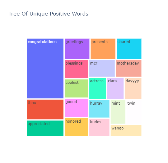
积极的推文

Unique_Positive= words_unique('positive', 20, raw_text)
print("The top 20 unique words in Positive Tweets are:")
Unique_Positive.style.background_gradient(cmap='Greens')

The top 20 unique words in Positive Tweets are:

Index	words	count
0	congratulations	29
1	thnx	10
2	appreciated	8
3	shared	7
4	presents	7
5	greetings	7
6	blessings	6
7	mothersday	6
8	mcr	6
9	coolest	6
10	honored	6
11	goood	6
12	wango	5
13	actress	5
14	mint	5
15	dayyyy	5
16	ciara	5
17	twin	5
18	kudos	5
19	hurray	5

fig = px.treemap(Unique_Positive, path=['words'], values='count',title='Tree Of Unique Positive Words')
fig.show()

from palettable.colorbrewer.qualitative import Pastel1_7
plt.figure(figsize=(16,10))
my_circle=plt.Circle((0,0), 0.7, color='white')
plt.pie(Unique_Positive['count'], labels=Unique_Positive.words, colors=Pastel1_7.hex_colors)
p=plt.gcf()
p.gca().add_artist(my_circle)
plt.title('DoNut Plot Of Unique Positive Words')
plt.show()

Unique_Negative= words_unique('negative', 10, raw_text)
print("The top 10 unique words in Negative Tweets are:")
Unique_Negative.style.background_gradient(cmap='Reds')

The top 10 unique words in Negative Tweets are:

Index	words	count
0	ache	12
1	suffering	9
2	allergic	7
3	cramps	7
4	saddest	7
5	pissing	7
6	sob	6
7	dealing	6
8	devastated	6
9	noes	6

from palettable.colorbrewer.qualitative import Pastel1_7
plt.figure(figsize=(16,10))
my_circle=plt.Circle((0,0), 0.7, color='white')
plt.rcParams['text.color'] = 'black'
plt.pie(Unique_Negative['count'], labels=Unique_Negative.words, colors=Pastel1_7.hex_colors)
p=plt.gcf()
p.gca().add_artist(my_circle)
plt.title('DoNut Plot Of Unique Negative Words')
plt.show()

Unique_Neutral= words_unique('neutral', 10, raw_text)
print("The top 10 unique words in Neutral Tweets are:")
Unique_Neutral.style.background_gradient(cmap='Oranges')

The top 10 unique words in Neutral Tweets are:

Index	words	count
0	settings	9
1	explain	7
2	mite	6
3	hiya	6
4	reader	5
5	pr	5
6	sorta	5
7	fathers	5
8	enterprise	5
9	guessed	5

from palettable.colorbrewer.qualitative import Pastel1_7
plt.figure(figsize=(16,10))
my_circle=plt.Circle((0,0), 0.7, color='white')
plt.pie(Unique_Neutral['count'], labels=Unique_Neutral.words, colors=Pastel1_7.hex_colors)
p=plt.gcf()
p.gca().add_artist(my_circle)
plt.title('DoNut Plot Of Unique Neutral Words')
plt.show()

通过查看每种情绪的独特单词，我们现在对数据有了更清晰的了解，这些独特的单词是推文情绪的强有力决定因素

词云图绘制

我们将按以下顺序构建词云：

中性推文的词云
积极推文的词云
负面推文的词云

def plot_wordcloud(text, mask=None, max_words=200, max_font_size=100, figure_size=(24.0,16.0), color = 'white',title = None, title_size=40, image_color=False):stopwords = set(STOPWORDS)more_stopwords = {'u', "im"}stopwords = stopwords.union(more_stopwords)wordcloud = WordCloud(background_color=color,stopwords = stopwords,max_words = max_words,max_font_size = max_font_size, random_state = 42,width=400, height=200,mask = mask)wordcloud.generate(str(text))plt.figure(figsize=figure_size)if image_color:image_colors = ImageColorGenerator(mask);plt.imshow(wordcloud.recolor(color_func=image_colors), interpolation="bilinear");plt.title(title, fontdict={'size': title_size,  'verticalalignment': 'bottom'})else:plt.imshow(wordcloud);plt.title(title, fontdict={'size': title_size, 'color': 'black', 'verticalalignment': 'bottom'})plt.axis('off');plt.tight_layout()  
d = '/kaggle/input/masks-for-wordclouds/'

我添加了更多单词，如 im 、 u （我们说这些单词出现在最常见的单词中，干扰了我们的分析）作为停用词

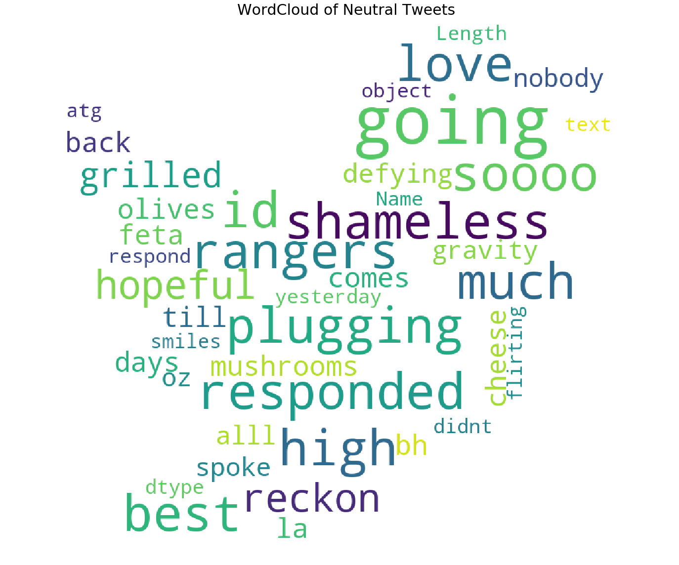
中性推文云

我们已经形象化了最常见的否定词，但词云为我们提供了更多的清晰度

pos_mask = np.array(Image.open(d+ 'twitter_mask.png'))
plot_wordcloud(Neutral_sent.text,mask=pos_mask,color='white',max_font_size=100,title_size=30,title="WordCloud of Neutral Tweets")

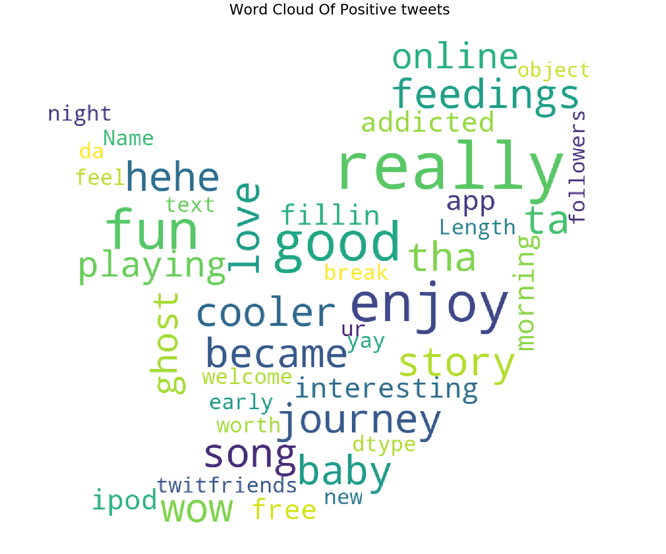
plot_wordcloud(Positive_sent.text,mask=pos_mask,title="Word Cloud Of Positive tweets",title_size=30)

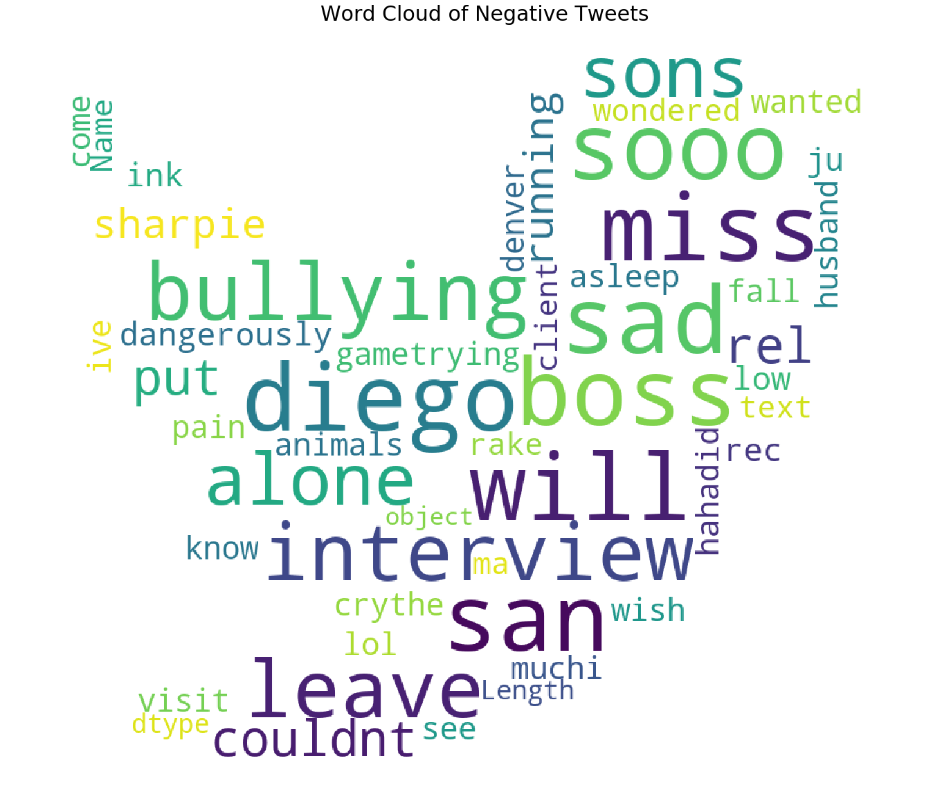
plot_wordcloud(Negative_sent.text,mask=pos_mask,title="Word Cloud of Negative Tweets",color='white',title_size=30)

模型构建

1) 将问题建模为 NER

命名实体识别 (NER) 是一个标准的 NLP 问题，涉及从文本块中识别命名实体（人物、地点、组织等），并将它们分类为一组预定义的类别。
为了理解 NER，这里有一篇非常好的文章：https://towardsdatascience.com/named-entity-recognition-with-nltk-and-spacy-8c4a7d88e7da

我们将使用 spacy 来创建我们自己的定制 NER 模型（针对每个情绪单独）。这种方法的动机当然是 Rohit Singh 共享的内核。

我的解决方案有何不同：

由于 jaccard 的高度相似性，我将使用文本作为所有中性推文的 selected_text
此外，我还将使用文本作为文本中字数少于 3 个的所有推文的 selected_text，如前所述
我将为正面和负面推文训练两种不同的模型
我不会预处理数据，因为所选文本包含原始文本

df_train = pd.read_csv('/kaggle/input/tweet-sentiment-extraction/train.csv')
df_test = pd.read_csv('/kaggle/input/tweet-sentiment-extraction/test.csv')
df_submission = pd.read_csv('/kaggle/input/tweet-sentiment-extraction/sample_submission.csv')

df_train['Num_words_text'] = df_train['text'].apply(lambda x:len(str(x).split())) #训练集中正文中的字数

df_train = df_train[df_train['Num_words_text']>=3]

要完全了解如何使用自定义输入训练 spacy NER，请阅读 spacy 文档以及本笔记本中的代码演示：https://spacy.io/usage/training#ner 按照更新 Spacy NER

def save_model(output_dir, nlp, new_model_name):''' This Function Saves model to given output directory'''output_dir = f'../working/{output_dir}'if output_dir is not None:        if not os.path.exists(output_dir):os.makedirs(output_dir)nlp.meta["name"] = new_model_namenlp.to_disk(output_dir)print("Saved model to", output_dir)

# 如果你想在现有模型上进行训练，请传递 model = nlpdef train(train_data, output_dir, n_iter=20, model=None):"""Load the model, set up the pipeline and train the entity recognizer."""""if model is not None:nlp = spacy.load(output_dir)  # load existing spaCy modelprint("Loaded model '%s'" % model)else:nlp = spacy.blank("en")  # create blank Language classprint("Created blank 'en' model")# 创建内置管道组件并将其添加到管道中# nlp.create_pipe 适用于在 spaCy 中注册的内置程序if "ner" not in nlp.pipe_names:ner = nlp.create_pipe("ner")nlp.add_pipe(ner, last=True)# 否则，获取它以便我们添加标签else:ner = nlp.get_pipe("ner")# 添加标签for _, annotations in train_data:for ent in annotations.get("entities"):ner.add_label(ent[2])# 获取其他管道的名称以在训练期间禁用它们other_pipes = [pipe for pipe in nlp.pipe_names if pipe != "ner"]with nlp.disable_pipes(*other_pipes):  # only train NER# sizes = compounding(1.0, 4.0, 1.001)# batch up the examples using spaCy's minibatchif model is None:nlp.begin_training()else:nlp.resume_training()for itn in tqdm(range(n_iter)):random.shuffle(train_data)batches = minibatch(train_data, size=compounding(4.0, 500.0, 1.001))    losses = {}for batch in batches:texts, annotations = zip(*batch)nlp.update(texts,  # batch of textsannotations,  # batch of annotationsdrop=0.5,   # dropout - make it harder to memorise datalosses=losses, )print("Losses", losses)save_model(output_dir, nlp, 'st_ner')

def get_model_out_path(sentiment):'''Returns Model output path'''model_out_path = Noneif sentiment == 'positive':model_out_path = 'models/model_pos'elif sentiment == 'negative':model_out_path = 'models/model_neg'return model_out_path

def get_training_data(sentiment):'''Returns Trainong data in the format needed to train spacy NER'''train_data = []for index, row in df_train.iterrows():if row.sentiment == sentiment:selected_text = row.selected_texttext = row.textstart = text.find(selected_text)end = start + len(selected_text)train_data.append((text, {"entities": [[start, end, 'selected_text']]}))return train_data

正面和负面推文的训练模型

sentiment = 'positive'train_data = get_training_data(sentiment)
model_path = get_model_out_path(sentiment)
# 出于演示目的，我进行了 3 次迭代，您可以根据需要训练模型
train(train_data, model_path, n_iter=3, model=None)

Created blank 'en' model33%|███▎      | 1/3 [00:52<01:45, 52.84s/it]Losses {'ner': 33900.41114743876}67%|██████▋   | 2/3 [01:45<00:52, 52.68s/it]Losses {'ner': 30517.31436416012}100%|██████████| 3/3 [02:37<00:00, 52.62s/it]Losses {'ner': 28912.80112953766}
Saved model to ../working/models/model_pos

sentiment = 'negative'train_data = get_training_data(sentiment)
model_path = get_model_out_path(sentiment)train(train_data, model_path, n_iter=3, model=None)

  0%|          | 0/3 [00:00<?, ?it/s]Created blank 'en' model33%|███▎      | 1/3 [00:50<01:41, 50.56s/it]Losses {'ner': 31926.559298905544}67%|██████▋   | 2/3 [01:40<00:50, 50.32s/it]Losses {'ner': 28526.67285699508}100%|██████████| 3/3 [02:30<00:00, 50.02s/it]Losses {'ner': 27071.952286979005}
Saved model to ../working/models/model_neg

使用经过训练的模型进行预测

def predict_entities(text, model):doc = model(text)ent_array = []for ent in doc.ents:start = text.find(ent.text)end = start + len(ent.text)new_int = [start, end, ent.label_]if new_int not in ent_array:ent_array.append([start, end, ent.label_])selected_text = text[ent_array[0][0]: ent_array[0][1]] if len(ent_array) > 0 else textreturn selected_text

selected_texts = []
MODELS_BASE_PATH = '../input/tse-spacy-model/models/'if MODELS_BASE_PATH is not None:print("Loading Models  from ", MODELS_BASE_PATH)model_pos = spacy.load(MODELS_BASE_PATH + 'model_pos')model_neg = spacy.load(MODELS_BASE_PATH + 'model_neg')for index, row in df_test.iterrows():text = row.textoutput_str = ""if row.sentiment == 'neutral' or len(text.split()) <= 2:selected_texts.append(text)elif row.sentiment == 'positive':selected_texts.append(predict_entities(text, model_pos))else:selected_texts.append(predict_entities(text, model_neg))df_test['selected_text'] = selected_texts

Loading Models  from  ../input/tse-spacy-model/models/

df_submission['selected_text'] = df_test['selected_text']
df_submission.to_csv("submission.csv", index=False)
display(df_submission.head(10))

Index	textID	selected_text
0	f87dea47db	Last session of the day http://twitpic.com/67ezh
1	96d74cb729	exciting
2	eee518ae67	Recession
3	01082688c6	happy bday!
4	33987a8ee5	I like it!!
5	726e501993	visitors!
6	261932614e	HATES
7	afa11da83f	blocked
8	e64208b4ef	and within a short time of the last clue all…
9	37bcad24ca	What did you get? My day is alright… haven’t…