改进系列(10):基于SwinTransformer+CBAM+多尺度特征融合+FocalLoss改进:自动驾驶地面路况识别
目录
1.代码介绍
1. 主训练脚本train.py
2. 工具函数与模型定义utils.py
3. GUI界面应用infer_QT.py
2.自动驾驶地面路况识别
3.训练过程
4.推理
5.下载
代码已经封装好,对小白友好。
想要更换数据集,参考readme文件摆放好数据集即可,可以一键训练!!
1.代码介绍
整体特点:
-
技术先进性:结合了Swin Transformer和注意力机制,利用了当前先进的深度学习技术。
-
完整流程:覆盖了从数据准备、模型训练到应用部署的完整流程。
-
模块化设计:各组件职责明确,耦合度低,便于维护和扩展。
-
可视化丰富:提供多种训练过程和数据分布的可视化,便于模型分析和调试。
-
用户友好:通过GUI界面降低了使用门槛,使技术成果更易于实际应用。
-
文档完整:代码结构清晰,注释充分,便于理解和二次开发。
这套系统适合作为图像分类任务的基础框架,可以根据具体需求进行调整和扩展,具有较强的实用性和灵活性。
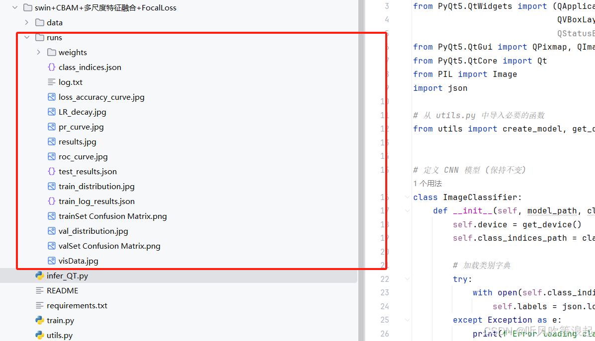
1. 主训练脚本train.py
train.py是系统的核心训练脚本,实现了完整的深度学习模型训练流程。
该脚本基于PyTorch框架,结合了Swin Transformer和CBAM注意力机制、多尺度特征融合,构建了一个强大的图像分类系统。
class SwinTransformerWithCBAM(nn.Module):def __init__(self, num_classes=10, pretrained=False):super(SwinTransformerWithCBAM, self).__init__()self.swin = models.swin_b(weights='IMAGENET1K_V1' if pretrained else None)# 获取各stage的实际输出通道数self.stage_channels = [128, 256, 512, 1024]# 添加CBAM模块self.cbam1 = CBAM(self.stage_channels[0])self.cbam2 = CBAM(self.stage_channels[1])self.cbam3 = CBAM(self.stage_channels[2])self.cbam4 = CBAM(self.stage_channels[3])# 多尺度特征融合self.multi_scale_fusion = MultiScaleFusion(in_channels_list=self.stage_channels,out_channels=256)# 分类头self.avgpool = nn.AdaptiveAvgPool2d(1)self.head = nn.Linear(256, num_classes)def forward(self, x):features = []# Stage 0: Patch Embeddingx = self.swin.features[0](x)# Stage 1x = self.swin.features[1](x)x = x.permute(0, 3, 1, 2) # (B, C, H, W)x = self.cbam1(x)features.append(x)x = x.permute(0, 2, 3, 1) # (B, H, W, C)# Stage 2x = self.swin.features[2](x) # Patch Mergingx = self.swin.features[3](x) # Stage2 blocksx = x.permute(0, 3, 1, 2)x = self.cbam2(x)features.append(x)x = x.permute(0, 2, 3, 1)# Stage 3x = self.swin.features[4](x) # Patch Mergingx = self.swin.features[5](x) # Stage3 blocksx = x.permute(0, 3, 1, 2)x = self.cbam3(x)features.append(x)x = x.permute(0, 2, 3, 1)# Stage 4x = self.swin.features[6](x) # Patch Mergingx = self.swin.features[7](x) # Stage4 blocksx = x.permute(0, 3, 1, 2)x = self.cbam4(x)features.append(x)# 多尺度特征融合fused_features = self.multi_scale_fusion(features)# 分类x = self.avgpool(fused_features[-1])x = torch.flatten(x, 1)x = self.head(x)return x主要功能包括:
-
参数配置与初始化:使用argparse模块处理命令行参数,包括模型选择、训练参数、数据路径等。创建保存结果的目录结构,记录训练配置信息。
-
数据准备:通过
data_trans()函数定义训练和验证数据的预处理流程,包括随机旋转、中心裁剪等增强操作。get_data()函数加载ImageFolder格式的数据集,并生成数据加载器。 -
模型构建:调用
create_model()函数创建Swin Transformer与CBAM、多尺度特征融合结合的混合模型,计算并记录模型参数量和计算量(FLOPs)。 -
训练流程:
- 使用Focal Loss作为损失函数,解决类别不平衡问题
- 实现余弦退火学习率调度策略
- 记录训练过程中的损失、准确率等指标
- 保存最佳模型和最后模型
-
评估与可视化:
- 绘制训练/验证的损失和准确率曲线
- 生成混淆矩阵
- 计算并绘制ROC曲线和PR曲线
- 可视化数据集分布
-
测试功能:可选地加载测试集进行最终评估,保存测试结果。
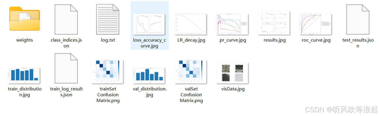
该脚本设计完整,包含了从数据准备到模型评估的完整流程,并提供了丰富的可视化功能,便于分析模型性能。
2. 工具函数与模型定义utils.py
utils.py包含了系统的主要工具函数和模型定义,是train和qt推理的基础支持模块。
主要组成部分:
-
注意力机制模块:
ChannelAttention:通道注意力模块,学习不同通道的重要性SpatialAttention:空间注意力模块,学习空间位置的重要性CBAM:结合通道和空间注意力的混合模块
-
多尺度特征融合:
MultiScaleFusion类实现了自顶向下的多尺度特征融合策略,增强模型对不同尺度特征的捕捉能力。 -
核心模型定义:
SwinTransformerWithCBAM类将Swin Transformer与CBAM注意力机制结合:- 使用预训练的Swin Transformer作为主干网络
- 在各阶段输出后添加CBAM模块
- 实现多尺度特征融合
- 自定义分类头
-
工具函数:
- 数据预处理(
data_trans) - 数据集加载(
get_data) - 训练和评估函数(
train_one_epoch,evaluate) - 混淆矩阵计算(
ConfusionMatrix) - 各种可视化函数(损失曲线、ROC曲线等)
- Focal Loss实现
- 数据预处理(
-
辅助功能:
- 目录创建(
mkdir) - 设备获取(
get_device) - 信息保存(
save_info) - 数据集分布可视化(
plot_dataset_distribution)
- 目录创建(
该文档提供了模型的核心实现和各种辅助工具,设计上注重模块化和可重用性,各组件可以方便地被其他脚本调用。
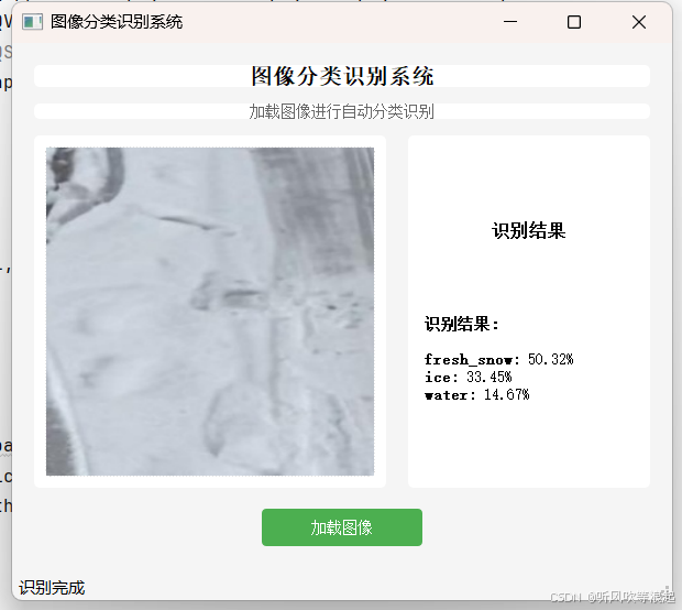
3. GUI界面应用infer_QT.py
infer_QT.py基于PyQt5实现了用户友好的图形界面,使训练好的模型可以方便地用于实际图像分类任务。
主要特点:
-
模型封装:
ImageClassifier类封装了模型加载和预测功能:- 从文件加载训练好的模型权重
- 加载类别标签映射文件
- 实现图像预处理和预测接口
-
GUI设计:
- 主窗口(
MainWindow)包含图像显示区、结果展示区和控制按钮 - 响应式布局,适应不同窗口大小
- 现代简洁的界面风格
- 状态栏显示操作状态
- 主窗口(
-
功能实现:
- 文件对话框选择图像
- 图像显示与自适应缩放
- 模型预测与结果显示(支持多类别概率展示)
- 错误处理和状态反馈
-
用户体验优化:
- 清晰的界面分区
- 操作状态反馈
- 美观的样式设计
- 详细的识别结果展示
该GUI应用使非技术用户也能方便地使用训练好的模型进行图像分类,提高了系统的实用性和易用性。
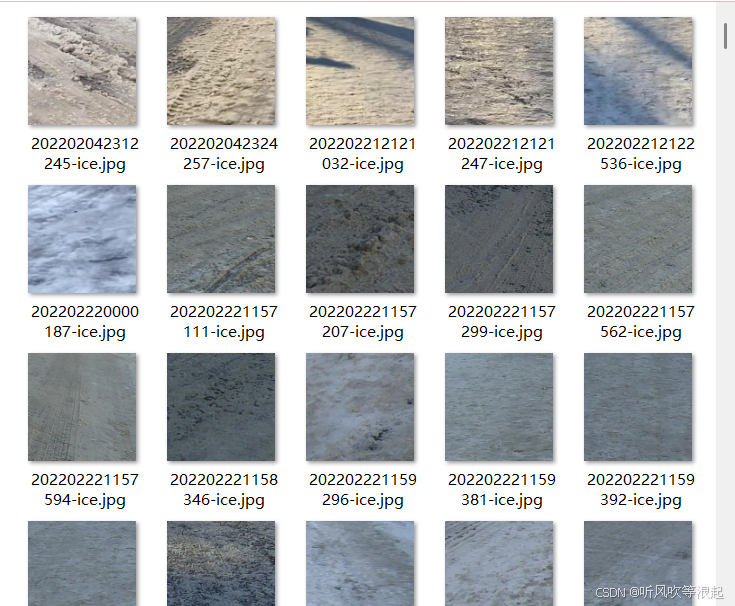
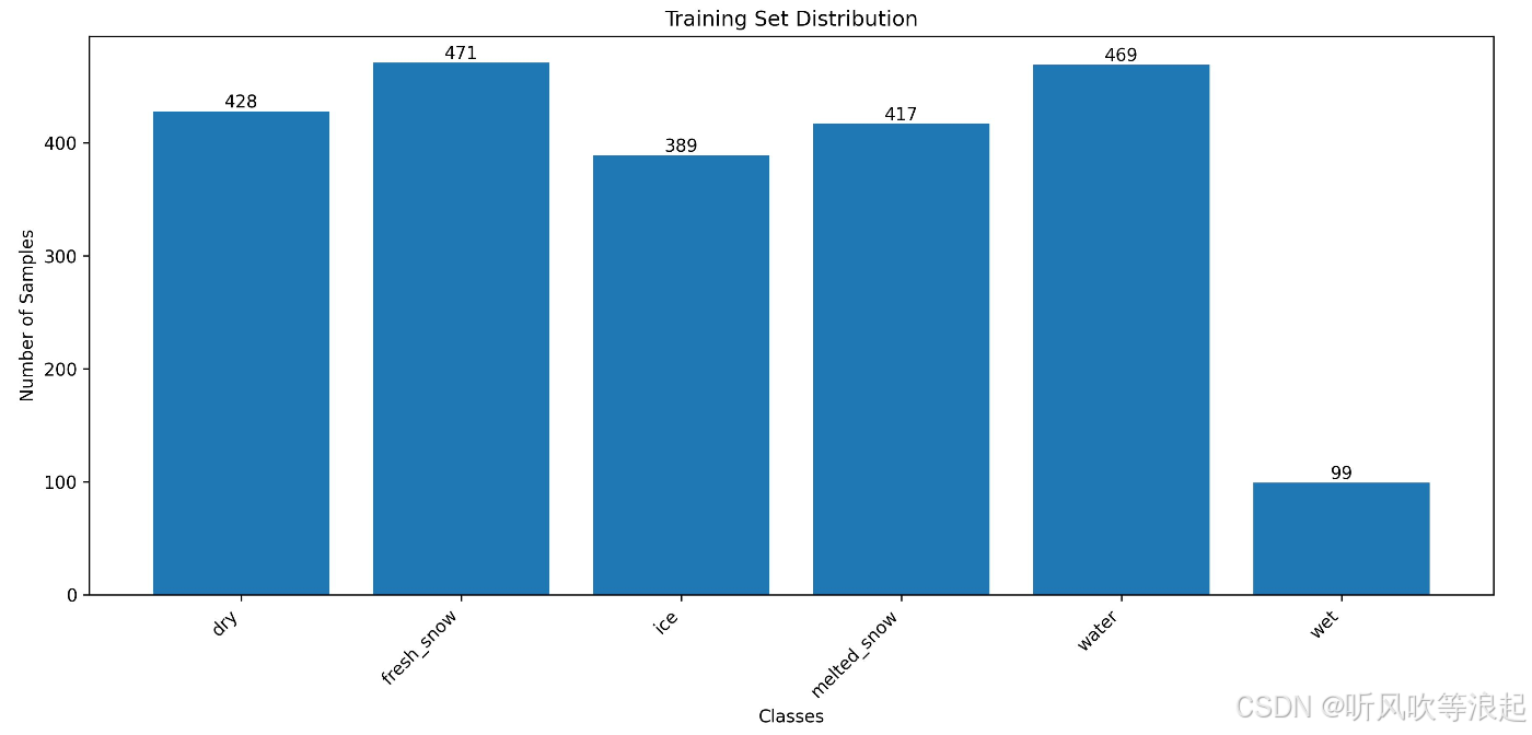
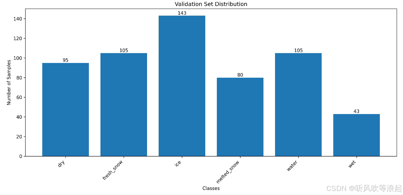
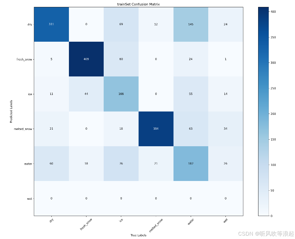
2.自动驾驶地面路况识别
数据集如下:
训练集和验证集的样本数量:【代码自动生成】
json标签:【代码自动生成】
{"0": "dry","1": "fresh_snow","2": "ice","3": "melted_snow","4": "water","5": "wet"
}
3.训练过程
参数如下:其实都很好理解的,就是常见的调参,这里不多介绍了
parser.add_argument("--model", default='swin-vit', type=str,help='swin-vit')parser.add_argument("--pretrained", default=False, type=bool) # 采用官方权重parser.add_argument("--batch-size", default=16, type=int)parser.add_argument("--epochs", default=5, type=int)parser.add_argument("--optim", default='Adam', type=str,help='SGD,Adam,AdamW') # 优化器选择parser.add_argument('--lr', default=0.0001, type=float)parser.add_argument('--lrf',default=0.0001,type=float) # 最终学习率 = lr * lrfparser.add_argument('--save_ret', default='runs', type=str) # 保存结果parser.add_argument('--data_train',default='./data/train',type=str) # 训练集路径parser.add_argument('--data_val',default='./data/val',type=str)# 测试集parser.add_argument("--data-test", default=True, type=bool, help='if exists test sets')数据集的文件摆放,有测试集的话,设置为true,代码会自动测试【参考readme文件】
--data--train--- 训练集的图像
--data--val--- 验证集的图像
--data--test--- 测试集的图像(如果有的话)
这里的loss采用focal loss:
class FocalLoss(nn.Module):def __init__(self, alpha=0.25, gamma=2.0, reduction='mean'):# 增大 gamma 会更强调难分类样本# 调整 alpha 可以平衡不同类别的权重super(FocalLoss, self).__init__()self.alpha = alphaself.gamma = gammaself.reduction = reductiondef forward(self, inputs, targets):ce_loss = F.cross_entropy(inputs, targets, reduction='none')pt = torch.exp(-ce_loss)focal_loss = self.alpha * (1-pt)**self.gamma * ce_lossif self.reduction == 'mean':return focal_loss.mean()elif self.reduction == 'sum':return focal_loss.sum()else:return focal_loss
训练日志:这里进行简单训练
Namespace(batch_size=16, data_test=True, data_train='./data/train', data_val='./data/val', epochs=5, lr=0.0001, lrf=0.0001, model='swin-vit', optim='Adam', pretrained=False, save_ret='runs')
Using device is: cuda
Using dataloader workers is : 8
trainSet number is : 2273 valSet number is : 571
model output is : 6
SwinTransformerWithCBAM((swin): SwinTransformer((features): Sequential((0): Sequential((0): Conv2d(3, 128, kernel_size=(4, 4), stride=(4, 4))(1): Permute()(2): LayerNorm((128,), eps=1e-05, elementwise_affine=True))(1): Sequential((0): SwinTransformerBlock((norm1): LayerNorm((128,), eps=1e-05, elementwise_affine=True)(attn): ShiftedWindowAttention((qkv): Linear(in_features=128, out_features=384, bias=True)(proj): Linear(in_features=128, out_features=128, bias=True))(stochastic_depth): StochasticDepth(p=0.0, mode=row)(norm2): LayerNorm((128,), eps=1e-05, elementwise_affine=True)(mlp): MLP((0): Linear(in_features=128, out_features=512, bias=True)(1): GELU(approximate='none')(2): Dropout(p=0.0, inplace=False)(3): Linear(in_features=512, out_features=128, bias=True)(4): Dropout(p=0.0, inplace=False)))(1): SwinTransformerBlock((norm1): LayerNorm((128,), eps=1e-05, elementwise_affine=True)(attn): ShiftedWindowAttention((qkv): Linear(in_features=128, out_features=384, bias=True)(proj): Linear(in_features=128, out_features=128, bias=True))(stochastic_depth): StochasticDepth(p=0.021739130434782608, mode=row)(norm2): LayerNorm((128,), eps=1e-05, elementwise_affine=True)(mlp): MLP((0): Linear(in_features=128, out_features=512, bias=True)(1): GELU(approximate='none')(2): Dropout(p=0.0, inplace=False)(3): Linear(in_features=512, out_features=128, bias=True)(4): Dropout(p=0.0, inplace=False))))(2): PatchMerging((reduction): Linear(in_features=512, out_features=256, bias=False)(norm): LayerNorm((512,), eps=1e-05, elementwise_affine=True))(3): Sequential((0): SwinTransformerBlock((norm1): LayerNorm((256,), eps=1e-05, elementwise_affine=True)(attn): ShiftedWindowAttention((qkv): Linear(in_features=256, out_features=768, bias=True)(proj): Linear(in_features=256, out_features=256, bias=True))(stochastic_depth): StochasticDepth(p=0.043478260869565216, mode=row)(norm2): LayerNorm((256,), eps=1e-05, elementwise_affine=True)(mlp): MLP((0): Linear(in_features=256, out_features=1024, bias=True)(1): GELU(approximate='none')(2): Dropout(p=0.0, inplace=False)(3): Linear(in_features=1024, out_features=256, bias=True)(4): Dropout(p=0.0, inplace=False)))(1): SwinTransformerBlock((norm1): LayerNorm((256,), eps=1e-05, elementwise_affine=True)(attn): ShiftedWindowAttention((qkv): Linear(in_features=256, out_features=768, bias=True)(proj): Linear(in_features=256, out_features=256, bias=True))(stochastic_depth): StochasticDepth(p=0.06521739130434782, mode=row)(norm2): LayerNorm((256,), eps=1e-05, elementwise_affine=True)(mlp): MLP((0): Linear(in_features=256, out_features=1024, bias=True)(1): GELU(approximate='none')(2): Dropout(p=0.0, inplace=False)(3): Linear(in_features=1024, out_features=256, bias=True)(4): Dropout(p=0.0, inplace=False))))(4): PatchMerging((reduction): Linear(in_features=1024, out_features=512, bias=False)(norm): LayerNorm((1024,), eps=1e-05, elementwise_affine=True))(5): Sequential((0): SwinTransformerBlock((norm1): LayerNorm((512,), eps=1e-05, elementwise_affine=True)(attn): ShiftedWindowAttention((qkv): Linear(in_features=512, out_features=1536, bias=True)(proj): Linear(in_features=512, out_features=512, bias=True))(stochastic_depth): StochasticDepth(p=0.08695652173913043, mode=row)(norm2): LayerNorm((512,), eps=1e-05, elementwise_affine=True)(mlp): MLP((0): Linear(in_features=512, out_features=2048, bias=True)(1): GELU(approximate='none')(2): Dropout(p=0.0, inplace=False)(3): Linear(in_features=2048, out_features=512, bias=True)(4): Dropout(p=0.0, inplace=False)))(1): SwinTransformerBlock((norm1): LayerNorm((512,), eps=1e-05, elementwise_affine=True)(attn): ShiftedWindowAttention((qkv): Linear(in_features=512, out_features=1536, bias=True)(proj): Linear(in_features=512, out_features=512, bias=True))(stochastic_depth): StochasticDepth(p=0.10869565217391304, mode=row)(norm2): LayerNorm((512,), eps=1e-05, elementwise_affine=True)(mlp): MLP((0): Linear(in_features=512, out_features=2048, bias=True)(1): GELU(approximate='none')(2): Dropout(p=0.0, inplace=False)(3): Linear(in_features=2048, out_features=512, bias=True)(4): Dropout(p=0.0, inplace=False)))(2): SwinTransformerBlock((norm1): LayerNorm((512,), eps=1e-05, elementwise_affine=True)(attn): ShiftedWindowAttention((qkv): Linear(in_features=512, out_features=1536, bias=True)(proj): Linear(in_features=512, out_features=512, bias=True))(stochastic_depth): StochasticDepth(p=0.13043478260869565, mode=row)(norm2): LayerNorm((512,), eps=1e-05, elementwise_affine=True)(mlp): MLP((0): Linear(in_features=512, out_features=2048, bias=True)(1): GELU(approximate='none')(2): Dropout(p=0.0, inplace=False)(3): Linear(in_features=2048, out_features=512, bias=True)(4): Dropout(p=0.0, inplace=False)))(3): SwinTransformerBlock((norm1): LayerNorm((512,), eps=1e-05, elementwise_affine=True)(attn): ShiftedWindowAttention((qkv): Linear(in_features=512, out_features=1536, bias=True)(proj): Linear(in_features=512, out_features=512, bias=True))(stochastic_depth): StochasticDepth(p=0.15217391304347827, mode=row)(norm2): LayerNorm((512,), eps=1e-05, elementwise_affine=True)(mlp): MLP((0): Linear(in_features=512, out_features=2048, bias=True)(1): GELU(approximate='none')(2): Dropout(p=0.0, inplace=False)(3): Linear(in_features=2048, out_features=512, bias=True)(4): Dropout(p=0.0, inplace=False)))(4): SwinTransformerBlock((norm1): LayerNorm((512,), eps=1e-05, elementwise_affine=True)(attn): ShiftedWindowAttention((qkv): Linear(in_features=512, out_features=1536, bias=True)(proj): Linear(in_features=512, out_features=512, bias=True))(stochastic_depth): StochasticDepth(p=0.17391304347826086, mode=row)(norm2): LayerNorm((512,), eps=1e-05, elementwise_affine=True)(mlp): MLP((0): Linear(in_features=512, out_features=2048, bias=True)(1): GELU(approximate='none')(2): Dropout(p=0.0, inplace=False)(3): Linear(in_features=2048, out_features=512, bias=True)(4): Dropout(p=0.0, inplace=False)))(5): SwinTransformerBlock((norm1): LayerNorm((512,), eps=1e-05, elementwise_affine=True)(attn): ShiftedWindowAttention((qkv): Linear(in_features=512, out_features=1536, bias=True)(proj): Linear(in_features=512, out_features=512, bias=True))(stochastic_depth): StochasticDepth(p=0.1956521739130435, mode=row)(norm2): LayerNorm((512,), eps=1e-05, elementwise_affine=True)(mlp): MLP((0): Linear(in_features=512, out_features=2048, bias=True)(1): GELU(approximate='none')(2): Dropout(p=0.0, inplace=False)(3): Linear(in_features=2048, out_features=512, bias=True)(4): Dropout(p=0.0, inplace=False)))(6): SwinTransformerBlock((norm1): LayerNorm((512,), eps=1e-05, elementwise_affine=True)(attn): ShiftedWindowAttention((qkv): Linear(in_features=512, out_features=1536, bias=True)(proj): Linear(in_features=512, out_features=512, bias=True))(stochastic_depth): StochasticDepth(p=0.21739130434782608, mode=row)(norm2): LayerNorm((512,), eps=1e-05, elementwise_affine=True)(mlp): MLP((0): Linear(in_features=512, out_features=2048, bias=True)(1): GELU(approximate='none')(2): Dropout(p=0.0, inplace=False)(3): Linear(in_features=2048, out_features=512, bias=True)(4): Dropout(p=0.0, inplace=False)))(7): SwinTransformerBlock((norm1): LayerNorm((512,), eps=1e-05, elementwise_affine=True)(attn): ShiftedWindowAttention((qkv): Linear(in_features=512, out_features=1536, bias=True)(proj): Linear(in_features=512, out_features=512, bias=True))(stochastic_depth): StochasticDepth(p=0.2391304347826087, mode=row)(norm2): LayerNorm((512,), eps=1e-05, elementwise_affine=True)(mlp): MLP((0): Linear(in_features=512, out_features=2048, bias=True)(1): GELU(approximate='none')(2): Dropout(p=0.0, inplace=False)(3): Linear(in_features=2048, out_features=512, bias=True)(4): Dropout(p=0.0, inplace=False)))(8): SwinTransformerBlock((norm1): LayerNorm((512,), eps=1e-05, elementwise_affine=True)(attn): ShiftedWindowAttention((qkv): Linear(in_features=512, out_features=1536, bias=True)(proj): Linear(in_features=512, out_features=512, bias=True))(stochastic_depth): StochasticDepth(p=0.2608695652173913, mode=row)(norm2): LayerNorm((512,), eps=1e-05, elementwise_affine=True)(mlp): MLP((0): Linear(in_features=512, out_features=2048, bias=True)(1): GELU(approximate='none')(2): Dropout(p=0.0, inplace=False)(3): Linear(in_features=2048, out_features=512, bias=True)(4): Dropout(p=0.0, inplace=False)))(9): SwinTransformerBlock((norm1): LayerNorm((512,), eps=1e-05, elementwise_affine=True)(attn): ShiftedWindowAttention((qkv): Linear(in_features=512, out_features=1536, bias=True)(proj): Linear(in_features=512, out_features=512, bias=True))(stochastic_depth): StochasticDepth(p=0.2826086956521739, mode=row)(norm2): LayerNorm((512,), eps=1e-05, elementwise_affine=True)(mlp): MLP((0): Linear(in_features=512, out_features=2048, bias=True)(1): GELU(approximate='none')(2): Dropout(p=0.0, inplace=False)(3): Linear(in_features=2048, out_features=512, bias=True)(4): Dropout(p=0.0, inplace=False)))(10): SwinTransformerBlock((norm1): LayerNorm((512,), eps=1e-05, elementwise_affine=True)(attn): ShiftedWindowAttention((qkv): Linear(in_features=512, out_features=1536, bias=True)(proj): Linear(in_features=512, out_features=512, bias=True))(stochastic_depth): StochasticDepth(p=0.30434782608695654, mode=row)(norm2): LayerNorm((512,), eps=1e-05, elementwise_affine=True)(mlp): MLP((0): Linear(in_features=512, out_features=2048, bias=True)(1): GELU(approximate='none')(2): Dropout(p=0.0, inplace=False)(3): Linear(in_features=2048, out_features=512, bias=True)(4): Dropout(p=0.0, inplace=False)))(11): SwinTransformerBlock((norm1): LayerNorm((512,), eps=1e-05, elementwise_affine=True)(attn): ShiftedWindowAttention((qkv): Linear(in_features=512, out_features=1536, bias=True)(proj): Linear(in_features=512, out_features=512, bias=True))(stochastic_depth): StochasticDepth(p=0.32608695652173914, mode=row)(norm2): LayerNorm((512,), eps=1e-05, elementwise_affine=True)(mlp): MLP((0): Linear(in_features=512, out_features=2048, bias=True)(1): GELU(approximate='none')(2): Dropout(p=0.0, inplace=False)(3): Linear(in_features=2048, out_features=512, bias=True)(4): Dropout(p=0.0, inplace=False)))(12): SwinTransformerBlock((norm1): LayerNorm((512,), eps=1e-05, elementwise_affine=True)(attn): ShiftedWindowAttention((qkv): Linear(in_features=512, out_features=1536, bias=True)(proj): Linear(in_features=512, out_features=512, bias=True))(stochastic_depth): StochasticDepth(p=0.34782608695652173, mode=row)(norm2): LayerNorm((512,), eps=1e-05, elementwise_affine=True)(mlp): MLP((0): Linear(in_features=512, out_features=2048, bias=True)(1): GELU(approximate='none')(2): Dropout(p=0.0, inplace=False)(3): Linear(in_features=2048, out_features=512, bias=True)(4): Dropout(p=0.0, inplace=False)))(13): SwinTransformerBlock((norm1): LayerNorm((512,), eps=1e-05, elementwise_affine=True)(attn): ShiftedWindowAttention((qkv): Linear(in_features=512, out_features=1536, bias=True)(proj): Linear(in_features=512, out_features=512, bias=True))(stochastic_depth): StochasticDepth(p=0.3695652173913043, mode=row)(norm2): LayerNorm((512,), eps=1e-05, elementwise_affine=True)(mlp): MLP((0): Linear(in_features=512, out_features=2048, bias=True)(1): GELU(approximate='none')(2): Dropout(p=0.0, inplace=False)(3): Linear(in_features=2048, out_features=512, bias=True)(4): Dropout(p=0.0, inplace=False)))(14): SwinTransformerBlock((norm1): LayerNorm((512,), eps=1e-05, elementwise_affine=True)(attn): ShiftedWindowAttention((qkv): Linear(in_features=512, out_features=1536, bias=True)(proj): Linear(in_features=512, out_features=512, bias=True))(stochastic_depth): StochasticDepth(p=0.391304347826087, mode=row)(norm2): LayerNorm((512,), eps=1e-05, elementwise_affine=True)(mlp): MLP((0): Linear(in_features=512, out_features=2048, bias=True)(1): GELU(approximate='none')(2): Dropout(p=0.0, inplace=False)(3): Linear(in_features=2048, out_features=512, bias=True)(4): Dropout(p=0.0, inplace=False)))(15): SwinTransformerBlock((norm1): LayerNorm((512,), eps=1e-05, elementwise_affine=True)(attn): ShiftedWindowAttention((qkv): Linear(in_features=512, out_features=1536, bias=True)(proj): Linear(in_features=512, out_features=512, bias=True))(stochastic_depth): StochasticDepth(p=0.41304347826086957, mode=row)(norm2): LayerNorm((512,), eps=1e-05, elementwise_affine=True)(mlp): MLP((0): Linear(in_features=512, out_features=2048, bias=True)(1): GELU(approximate='none')(2): Dropout(p=0.0, inplace=False)(3): Linear(in_features=2048, out_features=512, bias=True)(4): Dropout(p=0.0, inplace=False)))(16): SwinTransformerBlock((norm1): LayerNorm((512,), eps=1e-05, elementwise_affine=True)(attn): ShiftedWindowAttention((qkv): Linear(in_features=512, out_features=1536, bias=True)(proj): Linear(in_features=512, out_features=512, bias=True))(stochastic_depth): StochasticDepth(p=0.43478260869565216, mode=row)(norm2): LayerNorm((512,), eps=1e-05, elementwise_affine=True)(mlp): MLP((0): Linear(in_features=512, out_features=2048, bias=True)(1): GELU(approximate='none')(2): Dropout(p=0.0, inplace=False)(3): Linear(in_features=2048, out_features=512, bias=True)(4): Dropout(p=0.0, inplace=False)))(17): SwinTransformerBlock((norm1): LayerNorm((512,), eps=1e-05, elementwise_affine=True)(attn): ShiftedWindowAttention((qkv): Linear(in_features=512, out_features=1536, bias=True)(proj): Linear(in_features=512, out_features=512, bias=True))(stochastic_depth): StochasticDepth(p=0.45652173913043476, mode=row)(norm2): LayerNorm((512,), eps=1e-05, elementwise_affine=True)(mlp): MLP((0): Linear(in_features=512, out_features=2048, bias=True)(1): GELU(approximate='none')(2): Dropout(p=0.0, inplace=False)(3): Linear(in_features=2048, out_features=512, bias=True)(4): Dropout(p=0.0, inplace=False))))(6): PatchMerging((reduction): Linear(in_features=2048, out_features=1024, bias=False)(norm): LayerNorm((2048,), eps=1e-05, elementwise_affine=True))(7): Sequential((0): SwinTransformerBlock((norm1): LayerNorm((1024,), eps=1e-05, elementwise_affine=True)(attn): ShiftedWindowAttention((qkv): Linear(in_features=1024, out_features=3072, bias=True)(proj): Linear(in_features=1024, out_features=1024, bias=True))(stochastic_depth): StochasticDepth(p=0.4782608695652174, mode=row)(norm2): LayerNorm((1024,), eps=1e-05, elementwise_affine=True)(mlp): MLP((0): Linear(in_features=1024, out_features=4096, bias=True)(1): GELU(approximate='none')(2): Dropout(p=0.0, inplace=False)(3): Linear(in_features=4096, out_features=1024, bias=True)(4): Dropout(p=0.0, inplace=False)))(1): SwinTransformerBlock((norm1): LayerNorm((1024,), eps=1e-05, elementwise_affine=True)(attn): ShiftedWindowAttention((qkv): Linear(in_features=1024, out_features=3072, bias=True)(proj): Linear(in_features=1024, out_features=1024, bias=True))(stochastic_depth): StochasticDepth(p=0.5, mode=row)(norm2): LayerNorm((1024,), eps=1e-05, elementwise_affine=True)(mlp): MLP((0): Linear(in_features=1024, out_features=4096, bias=True)(1): GELU(approximate='none')(2): Dropout(p=0.0, inplace=False)(3): Linear(in_features=4096, out_features=1024, bias=True)(4): Dropout(p=0.0, inplace=False)))))(norm): LayerNorm((1024,), eps=1e-05, elementwise_affine=True)(permute): Permute()(avgpool): AdaptiveAvgPool2d(output_size=1)(flatten): Flatten(start_dim=1, end_dim=-1)(head): Linear(in_features=1024, out_features=1000, bias=True))(cbam1): CBAM((ca): ChannelAttention((avg_pool): AdaptiveAvgPool2d(output_size=1)(max_pool): AdaptiveMaxPool2d(output_size=1)(fc1): Conv2d(128, 8, kernel_size=(1, 1), stride=(1, 1), bias=False)(relu1): ReLU()(fc2): Conv2d(8, 128, kernel_size=(1, 1), stride=(1, 1), bias=False)(sigmoid): Sigmoid())(sa): SpatialAttention((conv): Conv2d(2, 1, kernel_size=(7, 7), stride=(1, 1), padding=(3, 3), bias=False)(sigmoid): Sigmoid()))(cbam2): CBAM((ca): ChannelAttention((avg_pool): AdaptiveAvgPool2d(output_size=1)(max_pool): AdaptiveMaxPool2d(output_size=1)(fc1): Conv2d(256, 16, kernel_size=(1, 1), stride=(1, 1), bias=False)(relu1): ReLU()(fc2): Conv2d(16, 256, kernel_size=(1, 1), stride=(1, 1), bias=False)(sigmoid): Sigmoid())(sa): SpatialAttention((conv): Conv2d(2, 1, kernel_size=(7, 7), stride=(1, 1), padding=(3, 3), bias=False)(sigmoid): Sigmoid()))(cbam3): CBAM((ca): ChannelAttention((avg_pool): AdaptiveAvgPool2d(output_size=1)(max_pool): AdaptiveMaxPool2d(output_size=1)(fc1): Conv2d(512, 32, kernel_size=(1, 1), stride=(1, 1), bias=False)(relu1): ReLU()(fc2): Conv2d(32, 512, kernel_size=(1, 1), stride=(1, 1), bias=False)(sigmoid): Sigmoid())(sa): SpatialAttention((conv): Conv2d(2, 1, kernel_size=(7, 7), stride=(1, 1), padding=(3, 3), bias=False)(sigmoid): Sigmoid()))(cbam4): CBAM((ca): ChannelAttention((avg_pool): AdaptiveAvgPool2d(output_size=1)(max_pool): AdaptiveMaxPool2d(output_size=1)(fc1): Conv2d(1024, 64, kernel_size=(1, 1), stride=(1, 1), bias=False)(relu1): ReLU()(fc2): Conv2d(64, 1024, kernel_size=(1, 1), stride=(1, 1), bias=False)(sigmoid): Sigmoid())(sa): SpatialAttention((conv): Conv2d(2, 1, kernel_size=(7, 7), stride=(1, 1), padding=(3, 3), bias=False)(sigmoid): Sigmoid()))(multi_scale_fusion): MultiScaleFusion((lateral_convs): ModuleList((0): Conv2d(128, 256, kernel_size=(1, 1), stride=(1, 1))(1): Conv2d(256, 256, kernel_size=(1, 1), stride=(1, 1))(2): Conv2d(512, 256, kernel_size=(1, 1), stride=(1, 1))(3): Conv2d(1024, 256, kernel_size=(1, 1), stride=(1, 1)))(fusion_convs): ModuleList((0-3): 4 x Conv2d(256, 256, kernel_size=(3, 3), stride=(1, 1), padding=(1, 1))))(avgpool): AdaptiveAvgPool2d(output_size=1)(head): Linear(in_features=256, out_features=6, bias=True)
)
[INFO] Register count_convNd() for <class 'torch.nn.modules.conv.Conv2d'>.
[INFO] Register count_normalization() for <class 'torch.nn.modules.normalization.LayerNorm'>.
[INFO] Register zero_ops() for <class 'torch.nn.modules.container.Sequential'>.
[INFO] Register count_linear() for <class 'torch.nn.modules.linear.Linear'>.
[INFO] Register zero_ops() for <class 'torch.nn.modules.dropout.Dropout'>.
[INFO] Register count_adap_avgpool() for <class 'torch.nn.modules.pooling.AdaptiveAvgPool2d'>.
[INFO] Register zero_ops() for <class 'torch.nn.modules.pooling.AdaptiveMaxPool2d'>.
[INFO] Register zero_ops() for <class 'torch.nn.modules.activation.ReLU'>.
Total parameters is:90.80 M
Train parameters is:90797102
Flops:12872.67 M
use optim is : Adam开始训练...
train: 100%|██████████| 143/143 [01:32<00:00, 1.54it/s, accuracy=0.445, loss=0.174]
valid: 100%|██████████| 36/36 [00:29<00:00, 1.21it/s, accuracy=0.468, loss=0.0589]
[epoch:0/5]
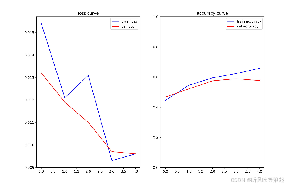
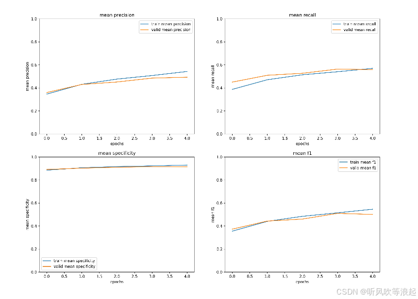
train loss:0.0154 train accuracy:0.4452
val loss:0.0132 val accuracy:0.4676train: 100%|██████████| 143/143 [01:31<00:00, 1.57it/s, accuracy=0.546, loss=0.121]
valid: 100%|██████████| 36/36 [00:29<00:00, 1.21it/s, accuracy=0.522, loss=0.0504]
train: 0%| | 0/143 [00:00<?, ?it/s][epoch:1/5]
train loss:0.0121 train accuracy:0.5460
val loss:0.0119 val accuracy:0.5219train: 100%|██████████| 143/143 [01:28<00:00, 1.62it/s, accuracy=0.594, loss=0.442]
valid: 100%|██████████| 36/36 [00:29<00:00, 1.24it/s, accuracy=0.574, loss=0.0512]
train: 0%| | 0/143 [00:00<?, ?it/s][epoch:2/5]
train loss:0.0131 train accuracy:0.5944
val loss:0.0110 val accuracy:0.5744train: 100%|██████████| 143/143 [01:27<00:00, 1.63it/s, accuracy=0.623, loss=0.0327]
valid: 100%|██████████| 36/36 [00:28<00:00, 1.24it/s, accuracy=0.588, loss=0.0539]
train: 0%| | 0/143 [00:00<?, ?it/s][epoch:3/5]
train loss:0.0093 train accuracy:0.6230
val loss:0.0097 val accuracy:0.5884train: 100%|██████████| 143/143 [01:27<00:00, 1.63it/s, accuracy=0.658, loss=0.202]
valid: 100%|██████████| 36/36 [00:29<00:00, 1.23it/s, accuracy=0.576, loss=0.0476]
[epoch:4/5]
train loss:0.0096 train accuracy:0.6582
val loss:0.0096 val accuracy:0.5762训练结束!!!
best epoch: 4
100%|██████████| 143/143 [00:37<00:00, 3.82it/s]
100%|██████████| 36/36 [00:25<00:00, 1.42it/s]
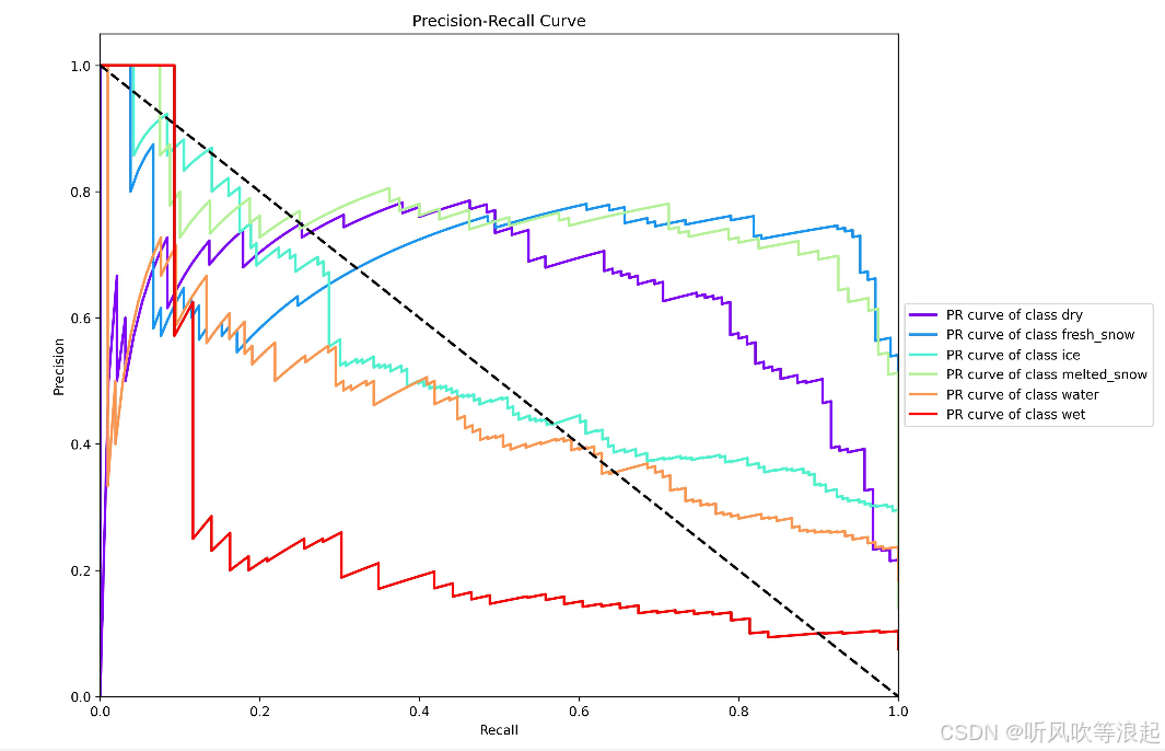
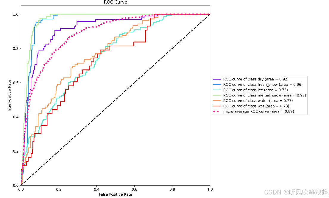
roc curve: 100%|██████████| 36/36 [00:25<00:00, 1.43it/s]
train finish!
验证集上表现最好的epoch为: 4
通过网络在测试集上进行测试valid: 0%| | 0/19 [00:00<?, ?it/s]6
['dry', 'fresh_snow', 'ice', 'melted_snow', 'water', 'wet']
valid: 100%|██████████| 19/19 [00:04<00:00, 4.13it/s, accuracy=0.543, loss=0.0382]
{'accuracy': 0.5427631578768828, 'dry': {'Precision': 0.5663, 'Recall': 0.7966, 'Specificity': 0.8531, 'F1 score': 0.662}, 'fresh_snow': {'Precision': 0.6481, 'Recall': 0.9211, 'Specificity': 0.9286, 'F1 score': 0.7609}, 'ice': {'Precision': 0.1429, 'Recall': 0.0435, 'Specificity': 0.9535, 'F1 score': 0.0667}, 'melted_snow': {'Precision': 0.6456, 'Recall': 0.8226, 'Specificity': 0.8843, 'F1 score': 0.7234}, 'water': {'Precision': 0.4054, 'Recall': 0.4478, 'Specificity': 0.8143, 'F1 score': 0.4255}, 'wet': {'Precision': 0.0, 'Recall': 0.0, 'Specificity': 1.0, 'F1 score': 0.0}, 'mean precision': 0.40138333333333326, 'mean recall': 0.5052666666666666, 'mean specificity': 0.9056333333333333, 'mean f1 score': 0.43975000000000003}
测试集的结果保存在---->test_results.json训练生成的文件:
{"train parameters": {"model version": "swin-vit","pretrained": false,"batch_size": 16,"epochs": 5,"optim": "Adam","lr": 0.0001,"lrf": 0.0001,"save_folder": "runs"},"dataset": {"trainset number": 2273,"valset number": 571,"number classes": 6},"model": {"total parameters": 90797102,"train parameters": 90797102,"flops": 12872672746.0},"epoch:0": {"train info": {"accuracy": 0.4452265728093039,"dry": {"Precision": 0.3983,"Recall": 0.4486,"Specificity": 0.8428,"F1 score": 0.422},"fresh_snow": {"Precision": 0.4553,"Recall": 0.6815,"Specificity": 0.7869,"F1 score": 0.5459},"ice": {"Precision": 0.3458,"Recall": 0.2134,"Specificity": 0.9167,"F1 score": 0.2639},"melted_snow": {"Precision": 0.6075,"Recall": 0.8129,"Specificity": 0.882,"F1 score": 0.6953},"water": {"Precision": 0.2683,"Recall": 0.1642,"Specificity": 0.8836,"F1 score": 0.2037},"wet": {"Precision": 0.0,"Recall": 0.0,"Specificity": 0.9995,"F1 score": 0.0},"mean precision": 0.3458666666666666,"mean recall": 0.3867666666666667,"mean specificity": 0.8852500000000001,"mean f1 score": 0.3551333333333333,"train loss": 0.0154},"valid info": {"accuracy": 0.46760070051720487,"dry": {"Precision": 0.4667,"Recall": 0.7368,"Specificity": 0.8319,"F1 score": 0.5714},"fresh_snow": {"Precision": 0.401,"Recall": 0.7905,"Specificity": 0.7339,"F1 score": 0.5321},"ice": {"Precision": 0.5301,"Recall": 0.3077,"Specificity": 0.9089,"F1 score": 0.3894},"melted_snow": {"Precision": 0.5929,"Recall": 0.8375,"Specificity": 0.9063,"F1 score": 0.6943},"water": {"Precision": 0.1667,"Recall": 0.0286,"Specificity": 0.9678,"F1 score": 0.0488},"wet": {"Precision": 0.0,"Recall": 0.0,"Specificity": 1.0,"F1 score": 0.0},"mean precision": 0.35956666666666665,"mean recall": 0.4501833333333333,"mean specificity": 0.8914666666666666,"mean f1 score": 0.37266666666666665,"val loss": 0.0132}},"epoch:1": {"train info": {"accuracy": 0.5459744830596306,"dry": {"Precision": 0.5168,"Recall": 0.5748,"Specificity": 0.8753,"F1 score": 0.5443},"fresh_snow": {"Precision": 0.6277,"Recall": 0.8662,"Specificity": 0.8657,"F1 score": 0.7279},"ice": {"Precision": 0.4167,"Recall": 0.2185,"Specificity": 0.9368,"F1 score": 0.2867},"melted_snow": {"Precision": 0.678,"Recall": 0.8585,"Specificity": 0.9084,"F1 score": 0.7576},"water": {"Precision": 0.347,"Recall": 0.307,"Specificity": 0.8498,"F1 score": 0.3258},"wet": {"Precision": 0.0,"Recall": 0.0,"Specificity": 1.0,"F1 score": 0.0},"mean precision": 0.4310333333333334,"mean recall": 0.47083333333333327,"mean specificity": 0.906,"mean f1 score": 0.44038333333333335,"train loss": 0.0121},"valid info": {"accuracy": 0.5218914185547829,"dry": {"Precision": 0.6087,"Recall": 0.5895,"Specificity": 0.9244,"F1 score": 0.5989},"fresh_snow": {"Precision": 0.5611,"Recall": 0.9619,"Specificity": 0.8305,"F1 score": 0.7088},"ice": {"Precision": 0.4222,"Recall": 0.1329,"Specificity": 0.9393,"F1 score": 0.2022},"melted_snow": {"Precision": 0.6228,"Recall": 0.8875,"Specificity": 0.9124,"F1 score": 0.732},"water": {"Precision": 0.3643,"Recall": 0.4857,"Specificity": 0.809,"F1 score": 0.4163},"wet": {"Precision": 0.0,"Recall": 0.0,"Specificity": 1.0,"F1 score": 0.0},"mean precision": 0.42985000000000007,"mean recall": 0.5095833333333334,"mean specificity": 0.9026000000000001,"mean f1 score": 0.4430333333333334,"val loss": 0.0119}},"epoch:2": {"train info": {"accuracy": 0.594368675756294,"dry": {"Precision": 0.5344,"Recall": 0.6893,"Specificity": 0.8607,"F1 score": 0.602},"fresh_snow": {"Precision": 0.6926,"Recall": 0.8896,"Specificity": 0.8968,"F1 score": 0.7788},"ice": {"Precision": 0.5,"Recall": 0.2751,"Specificity": 0.9432,"F1 score": 0.3549},"melted_snow": {"Precision": 0.728,"Recall": 0.8921,"Specificity": 0.9251,"F1 score": 0.8017},"water": {"Precision": 0.4041,"Recall": 0.3369,"Specificity": 0.8708,"F1 score": 0.3675},"wet": {"Precision": 0.0,"Recall": 0.0,"Specificity": 1.0,"F1 score": 0.0},"mean precision": 0.4765166666666667,"mean recall": 0.5138333333333334,"mean specificity": 0.9161000000000001,"mean f1 score": 0.48415,"train loss": 0.0131},"valid info": {"accuracy": 0.5744308231072779,"dry": {"Precision": 0.491,"Recall": 0.8632,"Specificity": 0.8214,"F1 score": 0.626},"fresh_snow": {"Precision": 0.8333,"Recall": 0.7143,"Specificity": 0.9678,"F1 score": 0.7692},"ice": {"Precision": 0.4762,"Recall": 0.6993,"Specificity": 0.743,"F1 score": 0.5666},"melted_snow": {"Precision": 0.7071,"Recall": 0.875,"Specificity": 0.9409,"F1 score": 0.7821},"water": {"Precision": 0.2,"Recall": 0.0095,"Specificity": 0.9914,"F1 score": 0.0181},"wet": {"Precision": 0.0,"Recall": 0.0,"Specificity": 1.0,"F1 score": 0.0},"mean precision": 0.4512666666666667,"mean recall": 0.5268833333333334,"mean specificity": 0.9107500000000001,"mean f1 score": 0.4603333333333333,"val loss": 0.011}},"epoch:3": {"train info": {"accuracy": 0.6229652441679588,"dry": {"Precision": 0.5638,"Recall": 0.785,"Specificity": 0.8591,"F1 score": 0.6563},"fresh_snow": {"Precision": 0.7576,"Recall": 0.8429,"Specificity": 0.9295,"F1 score": 0.798},"ice": {"Precision": 0.5523,"Recall": 0.3393,"Specificity": 0.9432,"F1 score": 0.4204},"melted_snow": {"Precision": 0.7421,"Recall": 0.9041,"Specificity": 0.9294,"F1 score": 0.8151},"water": {"Precision": 0.4286,"Recall": 0.371,"Specificity": 0.8714,"F1 score": 0.3977},"wet": {"Precision": 0.0,"Recall": 0.0,"Specificity": 1.0,"F1 score": 0.0},"mean precision": 0.5074,"mean recall": 0.5403833333333333,"mean specificity": 0.9221,"mean f1 score": 0.5145833333333333,"train loss": 0.0093},"valid info": {"accuracy": 0.5884413309879433,"dry": {"Precision": 0.5714,"Recall": 0.8,"Specificity": 0.8803,"F1 score": 0.6666},"fresh_snow": {"Precision": 0.7293,"Recall": 0.9238,"Specificity": 0.9227,"F1 score": 0.8151},"ice": {"Precision": 0.561,"Recall": 0.3217,"Specificity": 0.9159,"F1 score": 0.4089},"melted_snow": {"Precision": 0.6607,"Recall": 0.925,"Specificity": 0.9226,"F1 score": 0.7708},"water": {"Precision": 0.3874,"Recall": 0.4095,"Specificity": 0.8541,"F1 score": 0.3981},"wet": {"Precision": 0.0,"Recall": 0.0,"Specificity": 1.0,"F1 score": 0.0},"mean precision": 0.4849666666666666,"mean recall": 0.5633333333333334,"mean specificity": 0.9159333333333334,"mean f1 score": 0.5099166666666667,"val loss": 0.0097}},"epoch:4": {"train info": {"accuracy": 0.6581610206746231,"dry": {"Precision": 0.5916,"Recall": 0.7921,"Specificity": 0.8732,"F1 score": 0.6773},"fresh_snow": {"Precision": 0.8298,"Recall": 0.9108,"Specificity": 0.9512,"F1 score": 0.8684},"ice": {"Precision": 0.6278,"Recall": 0.3599,"Specificity": 0.9559,"F1 score": 0.4575},"melted_snow": {"Precision": 0.7451,"Recall": 0.9113,"Specificity": 0.93,"F1 score": 0.8199},"water": {"Precision": 0.4622,"Recall": 0.4435,"Specificity": 0.8659,"F1 score": 0.4527},"wet": {"Precision": 0.0,"Recall": 0.0,"Specificity": 1.0,"F1 score": 0.0},"mean precision": 0.54275,"mean recall": 0.5696,"mean specificity": 0.9293666666666667,"mean f1 score": 0.5459666666666667,"train loss": 0.0096},"valid info": {"accuracy": 0.5761821365923611,"dry": {"Precision": 0.5652,"Recall": 0.8211,"Specificity": 0.8739,"F1 score": 0.6695},"fresh_snow": {"Precision": 0.7252,"Recall": 0.9048,"Specificity": 0.9227,"F1 score": 0.8051},"ice": {"Precision": 0.6078,"Recall": 0.2168,"Specificity": 0.9533,"F1 score": 0.3196},"melted_snow": {"Precision": 0.7087,"Recall": 0.9125,"Specificity": 0.9389,"F1 score": 0.7978},"water": {"Precision": 0.3514,"Recall": 0.4952,"Specificity": 0.794,"F1 score": 0.4111},"wet": {"Precision": 0.0,"Recall": 0.0,"Specificity": 1.0,"F1 score": 0.0},"mean precision": 0.49305,"mean recall": 0.5584000000000001,"mean specificity": 0.9138000000000001,"mean f1 score": 0.5005166666666666,"val loss": 0.0096}}
}
这些都是代码自动生成的,摆放好数据集即可:
4.推理
这里使用QT推理:
5.下载
下载地址:Swin-Transformer+CBAM+多尺度特征融合+Focalloss改进:自动驾驶路面信息分类资源-CSDN文库
关于神经网络的改进,可以关注本人专栏:AI 改进系列_听风吹等浪起的博客-CSDN博客
相关文章:
改进系列(10):基于SwinTransformer+CBAM+多尺度特征融合+FocalLoss改进:自动驾驶地面路况识别
目录 1.代码介绍 1. 主训练脚本train.py 2. 工具函数与模型定义utils.py 3. GUI界面应用infer_QT.py 2.自动驾驶地面路况识别 3.训练过程 4.推理 5.下载 代码已经封装好,对小白友好。 想要更换数据集,参考readme文件摆放好数据集即可,…...

大型连锁酒店集团数据湖应用示例
目录 一、应用前面临的严峻背景 二、数据湖的精细化构建过程 (一)全域数据整合规划 (二)高效的数据摄取与存储架构搭建 (三)完善的元数据管理体系建设 (四)强大的数据分析平台…...
)
element.scrollIntoView(options)
handleNextClick 函数详解 功能描述 该函数实现在一个表格中“跳转到下一行”的功能,并将目标行滚动至视图顶部。通常用于导航或高亮显示当前选中的数据行。 const handleNextClick () > {// 如果当前已经是最后一行,则不执行后续操作if (current…...

python查看指定的进程是否存在
import os class Paly_Install(object):"""项目根目录"""def get_path(self):self.basedir os.path.dirname(os.path.abspath(__file__))"""安装失败的txt文件"""def test_app(self):self.app["com.faceboo…...

HAproxy+keepalived+tomcat部署高可用负载均衡实践
目录 一、前言 二、服务器规划 三、部署 1、jdk18安装 2、tomcat安装 3、haproxy安装 4、keepalived安装 三、测试 1、服务器停机测试 2、停止haproxy服务测试 总结 一、前言 HAProxy是一个使用C语言编写的自由及开放源代码软件,其提供高可用性、…...

C++负载均衡远程调用学习之自定义内存池管理
目录 1.内存管理_io_buf的结构分析 2.Lars_内存管理_io_buf内存块的实现 3.buf总结 4.buf_pool连接池的单例模式设计和基本属性 5.buf_pool的初始化构造内存池 6.buf_pool的申请内存和重置内存实现 7.课前回顾 1.内存管理_io_buf的结构分析 ## 3) Lars系统总体架构 …...

mysql-5.7.24-linux-glibc2.12-x86_64.tar.gz的下载安装和使用
资源获取链接: mysql-5.7.24-linux-glibc2.12-x86-64.tar.gz和使用说明资源-CSDN文库 详细作用 数据库服务器的核心文件: 这是一个压缩包,解压后包含 MySQL 数据库服务器的可执行文件、库文件、配置文件模板等。 它用于在 Linux 系统上安装…...

Kafka Producer的acks参数对消息可靠性有何影响?
1. acks0 可靠性最低生产者发送消息后不等待任何Broker确认可能丢失消息(Broker处理失败/网络丢失时无法感知)吞吐量最高,适用于允许数据丢失的场景(如日志收集) 2. acks1 (默认值) Leader副本确认模式生产者等待Le…...

Linux-04-用户管理命令
一、useradd添加新用户: 基本语法: useradd 用户名:添加新用户 useradd -g 组名 用户:添加新用户到某个组二、passwd设置用户密码: 基本语法: passwd 用户名:设置用户名密码 三、id查看用户是否存在: 基本语法: id 用户名 四、su切换用户: 基本语法: su 用户名称:切换用…...

node爬虫包 pup-crawler,超简单易用
PUP Crawler 这是一个基于puppeteer的简单的爬虫,可以爬取动态、静态加载的网站。 常用于【列表-详情-内容】系列的网站,比如电影视频等网站。 github地址 Usage npm install pup-crawler简单用法: import { PupCrawler } from pup-craw…...

艺术与科技的双向奔赴——高一鑫荣获加州联合表彰
2025年4月20日,在由M.A.D公司协办的“智艺相融,共赴价值巅峰”(Academic and Artistic Fusion Tribute to the Summit of Value)主题发布会上,音乐教育与科技融合领域的代表人物高一鑫,因其在数字音乐教育与中美文化交流方面的杰出贡献,荣获了圣盖博市议员Jorge Herrera和尔湾市…...

React-Native Android 多行被截断
1. 问题描述: 如图所示: 2. 问题解决灵感: 使用相同的react-native代码,运行在两个APP(demo 和 project)上。demo 展示正常,project 展示不正常。 对两个页面截图,对比如下。 得出…...

Canvas基础篇:图形绘制
Canvas基础篇:图形绘制 图形绘制moveTo()lineTo()lineTo绘制一条直线代码示例效果预览 lineTo绘制平行线代码示例效果预览 lineTo绘制矩形代码示例效果预览 arc()arc绘制一个圆代码实现效果预览 arc绘制一段弧代码实现效果预览 arcTo()rect()曲线 结语 图形绘制 在…...

自定义实现elementui的锚点
背景 前不久有个需求,上半部分是el-step步骤条,下半部分是一些文字说明,需要实现点击步骤条中某个步骤自定义定位到对应部分的文字说明,同时滚动内容区域的时候还要自动选中对应区域的步骤。element-ui-plus的有锚点这个组件&…...

基于UNet算法的农业遥感图像语义分割——补充版
前言 本案例希望建立一个UNET网络模型,来实现对农业遥感图像语义分割的任务。本篇博客主要包括对上一篇博客中的相关遗留问题进行解决,并对网络结构进行优化调整以适应个人的硬件设施——NVIDIA GeForce RTX 3050。 本案例的前两篇博客直达链接基于UNe…...

分布式数字身份:迈向Web3.0世界的通行证 | 北京行活动预告
数字经济浪潮奔涌向前,Web3.0发展方兴未艾,分布式数字身份(Decentralized Identity,简称DID)通过将分布式账本技术与身份治理相融合,在Web3.0时代多方协作的分布式应用场景中发挥核心作用,是构建…...

CentOS网络之network和NetworkManager深度解析
文章目录 CentOS网络之network和NetworkManager深度解析1. CentOS网络服务发展历史1.1 传统network阶段(CentOS 5-6)1.2 过渡期(CentOS 7)1.3 新时代(CentOS 8) 2. network和NetworkManager的核心区别3. ne…...

【XR】MR芯片 和 VR芯片之争
【XR】MR芯片 和 VR芯片之争 1. MR芯片 和 VR芯片 之间的最大差异是什么2. MR芯片 和 VR芯片 之间的最大差异是什么,国内外市场上有哪些芯片,价格如何,市场怎么样,芯片价格怎么样1. MR芯片 和 VR芯片 之间的最大差异是什么 MR芯片(混合现实芯片)与VR芯片(虚拟现实芯片)…...

关于安卓自动化打包docker+jenkins实现
背景 安卓开发过程中,尤其是提测后,会有一个发包的流程。这个流程简单来说,一般都是开发打包,然后发群里,测试再下载,发送到分发平台,然后把分发平台的应用主页发出来,最后群里面的…...

如何使用CAN分析仪验证MCU CAN错误机制
本文通过实验验证CAN控制器的错误处理机制是否符合相关标准。具体而言,我们使用ZPS-CANFD设备(ZPS-CANFD介绍)作为测量工具,USBCANFD-200U作为被测设备(DUT),通过注入特定类型的错误,…...

Centos 7安装 NVIDIA CUDA Toolkit
下载 # 查看操作系统信息 uname -m && cat /etc/redhat-release # 查看显卡信息 lspci | grep -i nvidia从NVIDIA CUDA Toolkit官网下载符合你需求的版本,我这里选择的是runfile(local)的方式。 安装 现在完成后进行安装 chmod x cuda_12.4.0_550.54.1…...

软件测试52讲学习分享:深入理解单元测试
课程背景 最近我在学习极客时间的《软件测试52讲》课程,这是由腾讯TEG基础架构部T4级专家茹炳晟老师主讲的认证课程。作为数字化转型与人工智能(DTAI)产业人才基地建设中心的认证课程,内容非常专业实用。今天想和大家分享第3讲"什么是单元测试&…...
 C#例子 Maui例子)
90.如何将Maui应用安装到手机(最简) C#例子 Maui例子
今天我来分享一下如何将Maui应用安装到手机上进行测试。 首先,创建一个新的Maui应用项目。 点击运行 在Visual Studio中,点击“运行”按钮,预览应用的初始效果,确保一切正常。 连接设备 使用数据线将手机连接到电脑。确保手机已…...

“100% 成功的 PyTorch CUDA GPU 支持” 安装攻略
#工作记录 一、总述 在深度学习领域,PyTorch 凭借其灵活性和强大的功能,成为了众多开发者和研究者的首选框架。而 CUDA GPU 支持能够显著加速 PyTorch 的计算过程,大幅提升训练和推理效率。然而,安装带有 CUDA GPU 支持的 PyTor…...

如何在Dify沙盒中安装运行pandas、numpy
如何在Dify沙盒中安装运行pandas、numpy 1. 创建python-requirements.txt文件2. 创建config.yaml文件3. 重启 docker-sandbox-14. 为什么要这样改的一些代码解析(Youtube视频截图) 1. 创建python-requirements.txt文件 在 Dify 的 Docker 目录下面&…...

ES集群搭建及工具类
文章说明 本文主要记录Windows下搭建ES集群的过程,并提供了一个通用的ES工具类;工具类采用http接口调用es功能,目前仅提供了简单的查询功能,可在基础上额外扩展 集群搭建 ES的下载安装非常简单,只需要下载软件的 zip 压…...
)
抓取工具Charles配置教程(mac电脑+ios手机)
mac电脑上的配置 1. 下载最新版本的Charles 2. 按照以下截图进行配置 2.1 端口号配置: 2.2 https配置 3. mac端证书配置 4. IOS手机端网络配置 4.1 先查看电脑上的配置 4.2 配置手机网络 连接和电脑同一个wifi,然后按照以下截图进行配置 5. 手机端证书…...

JavaScript 代码搜索框
1. 概述与需求分析 功能:在网页中实时搜索用户代码、关键字;展示匹配行、文件名;支持高亮、正则、模糊匹配。非功能:大文件集(几十万行)、高并发、响应 <100ms;支持增量索引和热更新。 2. …...

ESP32开发-作为TCP服务端接收数据
ESP32 ENC28J60 仅作为TCP服务端 (电脑通过 网络调试助手 连接ESP32,实现双向通信) 完整代码 #include <SPI.h> #include <EthernetENC.h> // 或 UIPEthernet.h// 网络配置 byte mac[] {0xDE, 0xAD…...
)
数智化招标采购系统针对供应商管理解决方案(采购如何管控供应商)
随着《优化营商环境条例》深化实施,采购领域正通过政策驱动和技术赋能,全面构建供应商全生命周期管理体系,以规范化、数智化推动采购生态向透明、高效、智能方向持续升级。 郑州信源数智化招标采购系统研发商,通过供应商管理子系…...

服务端字符过滤 与 SQL PDO防注入
注入示例 # step 1 SQL SELECT * FROM users WHERE username admin AND password e10adc3949ba59abbe56e057f20f883e # step 2 SQL SELECT * FROM users WHERE username admin# AND password 96e79218965eb72c92a549dd5a330112 关键点是这2个SQL的区别.其中第二步由于前台传…...

章越科技赋能消防训练体征监测与安全保障,从传统模式到智能跃迁的实践探索
引言:智能化转型浪潮下,消防训练的“破局”之需 2021年《“十四五”国家消防工作规划》的出台,标志着我国消防救援体系正式迈入“全灾种、大应急”的全新阶段。面对地震、洪涝、危化品泄漏等复杂救援场景,消防员不仅需要更强的体…...

RSYSLOG收集深信服log
RSYSLOG收集深信服ATRUST日志配置一直不成功,没有生成log文件,网上搜索到:如果你想要接收所有来自特定 IP 的日志,可以使用更通用的模式: 参考着修改配置 if $fromhost-ip 172.18.1.13 then /data/logs/network-devi…...

Golang - 实现文件管理服务器
先看效果: 代码如下: package mainimport ("fmt""html/template""log""net/http""os""path/filepath""strings" )// 配置根目录(根据需求修改) //var ba…...
里使用iview的注意事项)
在原生代码(非webpack)里使用iview的注意事项
最近公司在做一个项目,使用的框架是iview,使用过程中同事遇到一些问题,这些问题对于有些同学来说根本就不是问题,但总会有同学需要,为了帮助不太会用的同学快速找到问题,做了如下整理: 下载vue,iview.min.j…...
)
基于go的简单管理系统(增删改查)
package mainimport ("database/sql""fmt"_ "github.com/go-sql-driver/mysql" )var db *sql.DBtype user struct {id intname stringage int }// 建立连接 func initDB() (err error) {dsn : "root:123456tcp(127.0.0.1:3306)/mysqltes…...

Python 用一等函数重新审视“命令”设计模式
引言 在软件开发中,设计模式是解决常见问题的有效方法。“命令”设计模式旨在解耦调用操作的对象(调用者)和提供实现的对象(接收者)。本文将深入探讨“命令”模式,并介绍如何使用一等函数对其进行简化。 …...

pycharm导入同目录下文件未标红但报错ModuleNotFoundError
此贴仅为记录debug过程,为防后续再次遇见 问题 问题情境 复现文章模型,pycharm项目初次运行 问题描述 在导入同目录下其它文件夹中的python文件时,未标红,但运行时报错ModuleNotFoundError 报错信息 未找到该模块 Traceback …...
)
BOSS的收入 - 华为OD机试(A卷,Java题解)
华为OD机试题库《C》限时优惠 9.9 华为OD机试题库《Python》限时优惠 9.9 华为OD机试题库《JavaScript》限时优惠 9.9 代码不懂有疑问欢迎留言或私我们的VX:code5bug。 题目描述 一个 XX 产品行销总公司,只有一个 boss,其有若干一级分销&…...
)
Qt:(创建项目)
目录 1. 使⽤QtCreator新建项⽬ 1.1 新建项⽬ 1.2 选择项⽬模板 1.3 选择项⽬路径 1.4 选择构建系统 1.5 填写类信息设置界⾯ 编辑 1.6 选择语⾔和翻译⽂件 1.6 选择Qt套件 1.7 选择版本控制系统 1.8 最终效果 1. 使⽤QtCreator新建项⽬ 1.1 新建项⽬ 打开Qt…...
)
网络原理 - 12(HTTP/HTTPS - 3 - 响应)
目录 认识“状态码”(status code) 200 OK 404 Not Found 403 Forbidden 405 Method Not Allowed 500 Internal Server Error 504 Gateway Timeout 302 Move temporarily 301 Moved Permanently 418 I am a teaport 状态码小结: …...

OpenCV 4.7企业级开发实战:从图像处理到目标检测的全方位指南
简介 OpenCV作为工业级计算机视觉开发的核心工具库,其4.7版本在图像处理、视频分析和深度学习模型推理方面实现了显著优化。 本文将从零开始,系统讲解OpenCV 4.7的核心特性和功能更新,同时结合企业级应用场景,提供详细代码示例和实战项目,帮助读者掌握从基础图像处理到复…...
篇六:阅读与注释 QString 这个类,包含了 QString 类的 完整源码,也附上 QLatin1String 类的)
QT6 源(63)篇六:阅读与注释 QString 这个类,包含了 QString 类的 完整源码,也附上 QLatin1String 类的
(9)给出完整的源代码: #ifndef QSTRING_H #define QSTRING_H//验证了,没有此宏定义的 #if 不成立 #if defined(QT_NO_CAST_FROM_ASCII) && defined(QT_RESTRICTED_CAST_FROM_ASCII) #error QT_NO_CAST_FROM_ASCII a…...

PixONE 六维力传感器:赋能 OEM 机器人,12 自由度精准感知
The PixONE,一款为OEM设计的多模态12自由度机器人传感器,以其卓越的性能和广泛的适用性,正引领着机器人传感技术的革新。这款传感器不仅外观精致,达到IP68防护等级,易于消毒,而且其中心的大孔设计使得电缆和…...

nginx 解决跨域问题
本地用 8080 端口启动的服务访问后台API有跨域问题, from origin http://localhost:8080 has been blocked by CORS policy: Response to preflight request doesnt pass access control check: Redirect is not allowed for a preflight request. 其实用 9021 端…...
:打造 ES 新特性查询助手)
私有知识库 Coco AI 实战(五):打造 ES 新特性查询助手
有了实战(四)的经验,再打造个 ES 新特性查询助手就非常简单了。新的小助手使用的数据还是 ES 官方文档,模型设置也可沿用上次小助手的设置。 克隆小助手 我们进入 Coco Server 首页小助手菜单,选择“ES 索引参数查询…...

2025 新生 DL-FWI 培训
摘要: 本贴给出 8 次讨论式培训的提纲, 每次培训 1 小时. Basic concepts 1.1 Sesmic data processing – regular process 1.2 Full waveform inversion 1.3 Deep learning full waveform inversion Network structure 2.1 InversionNet Encoder-decorder structure 2.2 FCNV…...

VR汽车线束:汽车制造的新变革
汽车线束,作为汽车电路网络的主体,宛如汽车的 “神经网络”,承担着连接汽车各个部件、传输电力与信号的重任,对汽车的正常运行起着关键作用。从汽车的发动机到仪表盘,从传感器到各类电子设备,无一不是通过线…...
)
Centos离线安装Docker(无坑版)
1、下载并上传docker离线安装包 官方地址:安装包下载 2、上传到离线安装的服务器解压 tar -zxvf docker-28.1.1.tgz#拷贝解压二进制文件到相关目录 cp docker/* /usr/bin/ 3、创建docker启动文件 cat << EOF > /usr/lib/systemd/system/docker.servic…...

JConsole监控centos服务器中的springboot的服务
场景 在centos服务器中,有一个aa.jar的springboot服务,我想用JConsole监控它的JVM情况,具体怎么实现。 配置 Spring Boot 应用以启用 JMX 在java应用启动项进行配置 java -Djava.rmi.server.hostname=服务器IP -Dcom.sun.management.jmxremote=true \ -Dcom.sun.managem…...